Does Company Size Slow Revenue Growth? Gibrat's Law Test in Python

September 6, 2026

What’s the question?

Equity research applies a size discount by reflex. A company selling $200 billion a year is assumed to grow more slowly than one selling $2 billion, because the base is larger and the arithmetic of large numbers has to bite somewhere. It is built into most valuation models, which taper growth toward the economy’s rate as the company scales.

Gibrat’s law says the opposite. Robert Gibrat proposed in 1931 that a firm’s growth rate is independent of its size: growth arrives as a proportional shock, and a large firm draws its percentage growth from the same distribution as a small one. Under that law the size discount is a habit rather than a finding.

Filings settle it: fix a set of companies at a past date, measure the next five years of revenue, and see whether the starting size predicted anything.

The approach

Size is measured by revenue, not market capitalisation. Gibrat’s law concerns the size of the thing that grows, and a market capitalisation embeds the market’s own growth forecast, which would fold the answer into the question.

1. Take the S&P 500 roster as it stood on 31 December 2014 and again on 31 December 2019, keyed on entity identifiers rather than symbols, so a company that later changed ticker stays one company.
2. Pull annual and quarterly revenue for every member. The base year is the fiscal year ending in the roster year, the end year five calendar years later.
3. Drop Financials, since a bank’s or an insurer’s revenue is assembled from interest and premium lines rather than sales.
4. Require each anchor year’s annual revenue to agree with that year’s four quarterly filings within a factor of roughly 1.5. A year that fails describes a different business, usually after a divestiture restatement.
5. Annualise growth over the exact days between period ends, then regress the five-year compound growth rate on the base-10 logarithm of base revenue, alone and with sector fixed effects.

A company acquired or taken private mid-window carries no filing at the far end and no growth rate; 346 companies from the 2014 roster and 387 from the 2019 roster complete a pair. Two windows guard against reading one macro episode as a law.

Code

import numpy as np
import pandas as pd
import statsmodels.api as sm
import xfinlink as xfl
from scipy.stats import spearmanr

xfl.set_api_key("YOUR_API_KEY")  # free at https://xfinlink.com/signup

WINDOWS = [("2014-12-31", 2014, 2019), ("2019-12-31", 2019, 2024)]


def panel(as_of, y0, y1):
    roster = xfl.index("sp500", as_of=as_of).drop_duplicates("entity_id")
    ids = sorted(int(e) for e in roster["entity_id"].dropna())
    df = pd.concat(
        [xfl.fundamentals(entity_id=ids[i:i + 40], period_type="all",
                          start=f"{y0 - 1}-06-01", end=f"{y1 + 1}-06-30",
                          fields=["revenue"])
         for i in range(0, len(ids), 40)], ignore_index=True)

    ann = df[df["period_type"] == "annual"].copy()
    ann = ann.sort_values(["entity_id", "fiscal_year", "period_end"])
    ann = ann.drop_duplicates(["entity_id", "fiscal_year"], keep="last")
    ann["year"] = ann["period_end"].dt.year
    ann = ann.drop_duplicates(["entity_id", "year"], keep="last")
    ann = ann[ann["revenue"] > 0]

    qtr = df[(df["period_type"] == "quarterly") & df["revenue"].notna()]
    qsum = qtr.groupby(["entity_id", "fiscal_year"])["revenue"].agg(["sum", "size"])
    qsum = qsum[qsum["size"] == 4]["sum"].rename("qsum")
    ann = ann.merge(qsum, left_on=["entity_id", "fiscal_year"], right_index=True, how="left")
    ann = ann[ann["qsum"].isna()
              | ann["qsum"].between(0.67 * ann["revenue"], 1.5 * ann["revenue"])]

    m = (ann[ann["year"] == y0].set_index("entity_id")
         .join(ann[ann["year"] == y1].set_index("entity_id"),
               lsuffix="_b", rsuffix="_f", how="inner"))
    m = m[m["gics_sector_b"] != "Financials"]
    m["years"] = (m["period_end_f"] - m["period_end_b"]).dt.days / 365.25
    m = m[m["years"].between(4.0, 6.0)]
    m["cagr"] = (m["revenue_f"] / m["revenue_b"]) ** (1 / m["years"]) - 1
    m["log_size"] = np.log10(m["revenue_b"] * 1e6)
    m["quintile"] = pd.qcut(m["log_size"], 5, labels=[1, 2, 3, 4, 5])
    return len(ids), m


for as_of, y0, y1 in WINDOWS:
    n_roster, m = panel(as_of, y0, y1)
    plain = sm.OLS(m["cagr"], sm.add_constant(m[["log_size"]])).fit()
    dummies = pd.get_dummies(m["gics_sector_b"], drop_first=True, dtype=float)
    sector = sm.OLS(m["cagr"],
                    sm.add_constant(pd.concat([m[["log_size"]], dummies], axis=1))).fit()

    print(f"{y0}-{y1}: roster {n_roster}, in sample {len(m)}, "
          f"median revenue ${m['revenue_b'].median() / 1000:.1f}bn, "
          f"median CAGR {m['cagr'].median() * 100:.1f}%")
    for label, r in (("size only", plain), ("+ sector", sector)):
        print(f"  {label:<10} slope {r.params['log_size'] * 100:+.2f}pp per 10x  "
              f"t {r.tvalues['log_size']:.2f}  p {r.pvalues['log_size']:.4f}  "
              f"R2 {r.rsquared:.3f}")
    rho, p = spearmanr(m["log_size"], m["cagr"])
    within = m.groupby("gics_sector_b", observed=True).apply(
        lambda g: spearmanr(g["log_size"], g["cagr"])[0] if len(g) > 9 else np.nan,
        include_groups=False)
    print(f"  spearman {rho:+.3f} (p={p:.4f})   "
          f"median within sector {within.median():+.3f}")
    print(m.groupby("quintile", observed=True).agg(
        n=("cagr", "size"), median_revenue=("revenue_b", "median"),
        mean_cagr=("cagr", "mean"), sd_cagr=("cagr", "std")).round(4))

Full script with formatting and visualisation: does-company-size-slow-revenue-growth-python.py

Output

==========================================================================
DOES COMPANY SIZE SLOW REVENUE GROWTH?
Point-in-time S&P 500 rosters ex Financials, five-year forward revenue CAGR
==========================================================================
window            roster   in sample   median revenue   median CAGR
2014 to 2019         500         346           $9.3bn          2.5%
2019 to 2024         501         387          $10.3bn          5.1%

REVENUE CAGR REGRESSED ON log10(BASE REVENUE)
window          model                   slope per 10x       t        p      R2
2014 to 2019    size only                     -2.66pp   -2.73   0.0068   0.021
2014 to 2019    + sector fixed effects        -2.98pp   -3.14   0.0018   0.215
2019 to 2024    size only                     -1.36pp   -2.12   0.0344   0.012
2019 to 2024    + sector fixed effects        -1.22pp   -1.75   0.0814   0.070

RANK CORRELATION BETWEEN SIZE AND FORWARD GROWTH (Spearman)
2014 to 2019    all companies rho -0.195 (p=0.0003)   median within sector rho -0.141
2019 to 2024    all companies rho -0.117 (p=0.0213)   median within sector rho -0.163

MEAN FORWARD REVENUE CAGR BY SIZE QUINTILE (Q1 smallest)
window                 Q1       Q2       Q3       Q4       Q5   Q1 - Q5
2014 to 2019         4.3%     4.8%     3.1%    -0.4%     2.4%      2.0pp
2019 to 2024         8.3%     5.4%     5.4%     4.2%     5.3%      3.1pp

MEDIAN BASE REVENUE BY SIZE QUINTILE, $bn
window                 Q1       Q2       Q3       Q4       Q5
2014 to 2019          2.6      5.1      9.3     17.7     64.3
2019 to 2024          2.8      5.8     10.3     19.2     66.0

SPREAD OF FIVE-YEAR CAGR WITHIN EACH SIZE QUINTILE (standard deviation, pp)
window                 Q1       Q2       Q3       Q4       Q5
2014 to 2019         10.5     11.1      9.1      7.1      8.2
2019 to 2024          7.3      6.4      7.3      5.4      5.8

What this tells us

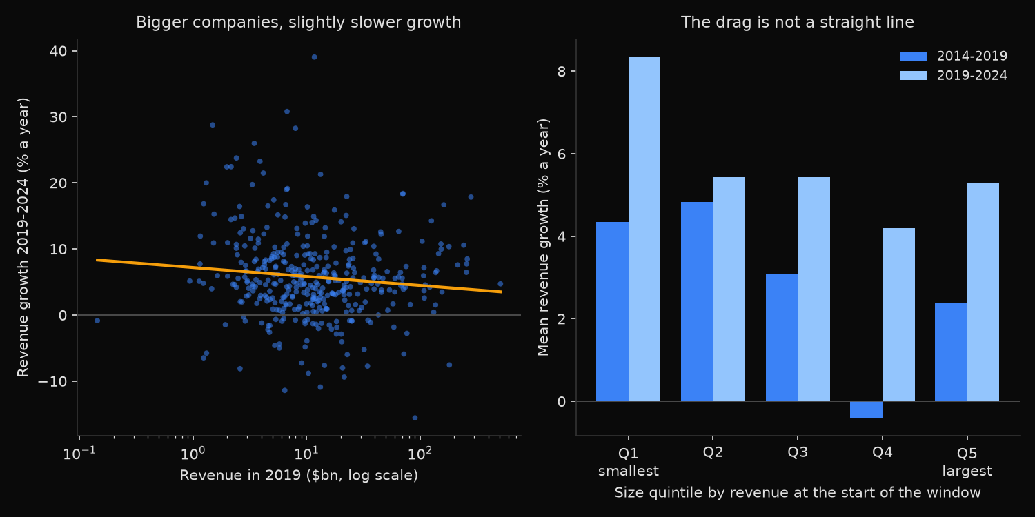
The size drag exists, and it is small. A tenfold increase in revenue costs 2.66 percentage points of annual growth in the 2014 window and 1.36 points in the 2019 window, both clearing the 5% threshold, with rank correlations of -0.195 and -0.117. R-squared is 0.021 and 0.012, so roughly 98% of the variation sits somewhere other than size, and growth within one quintile has a standard deviation of 5.4 to 11.1 points against gaps of 2.0 and 3.1 points between the smallest and largest fifths.

Sector is the bigger effect by an order of magnitude, lifting R-squared from 0.021 to 0.215 in the 2014 window. The size slope survives that control there, at -2.98 points with a t-statistic of -3.14, but in the 2019 window it weakens to -1.22 points and a p-value of 0.0814, short of conventional significance. Within-sector rank correlations of -0.141 and -0.163 run the same direction in both windows, so the drag is not merely small companies sitting in fast-growing industries; it is too weak for one window to confirm.

The quintile means break the folk version of the claim outright. In both windows the fourth quintile grew more slowly than the fifth: -0.4% against 2.4% in 2014-2019, and 4.2% against 5.3% in 2019-2024. Companies with a median of $64 billion in revenue outgrew companies with a median of $18 billion. The pattern is a fast-growing smallest fifth, 8.3% a year in the recent window, with the other four quintiles bunched between 4.2% and 5.4%: a step at the bottom of the size range, not a slope running its length.

So what?

Discounting a large company’s growth forecast on size alone takes a 1 to 3 point effect and ignores the 5 to 11 point dispersion around it. The penalty these regressions support is one to three points of growth per order of magnitude of revenue, and no more. Anything steeper is an assumption rather than an inference from the cross-section.

For growth screening the order is sector first, company second, size a distant third. A size filter drops most of the universe to buy a shift in expected growth smaller than the spread inside any bucket it leaves behind. Size earns attention at the bottom edge of the large-cap range, where the smallest fifth compounded 3.2 points a year faster than the quintiles above it in the recent window and 1.9 points faster in the earlier one.

Built with xfinlink — free financial data API for Python. pip install -U xfinlink