
What’s the question?
Sectors get sorted into cyclical and defensive, and the sorting is almost always done with share prices. A sector whose ETF falls harder than the market in a selloff is called cyclical; one that falls less is called defensive. That label then drives decisions about what to hold into a slowdown. Whether price-defined defensives limit losses without giving up gains is the test in an up and down capture analysis.
Stock beta measures how a sector’s shares move with the market, not how its business moves with the economy. Revenue beta measures the second thing: the sensitivity of a sector’s year-over-year sales growth to the sales growth of the rest of the corporate sector. A revenue beta of 2 means sector sales swing twice as far as the corporate average in both directions. Setting the two side by side asks whether the market’s cyclicality ranking matches the ranking inside the businesses.
The approach
Revenue rather than earnings, because it is the cleanest quarterly read on demand, ahead of operating leverage, tax and accounting choices.
- Rebuild S&P 500 membership at every quarter end from 2018Q3 to 2026Q1, addressing each company by entity id so a ticker change does not break the panel and a departing member stops contributing from the quarter it leaves.
- Pull quarterly revenue for every company that was a member at any point in the window. Financials and Real Estate are excluded: a bank’s revenue is an interest and fee aggregate, a REIT’s is contracted rent.
- Place each fiscal quarter in the calendar quarter it covers. Apple’s fiscal Q3 in 2023 ended on 1 July and its Q4 on 30 September, so both period ends fall inside calendar Q3.
- Compute each company’s revenue growth against the same quarter a year earlier. The sector line is the median growth across that sector’s index members, and the cycle line is the median across every member outside it, so one spin-off cannot move a sector.
- Regress each sector line on its cycle line with Newey-West standard errors at four lags, since year-over-year growth sampled quarterly overlaps by three quarters. The slope is the revenue beta.
- Estimate each sector ETF’s stock beta against SPY from daily returns over the same window.
Code
import pandas as pd
import statsmodels.api as sm
import xfinlink as xfl

xfl.set_api_key("YOUR_API_KEY")  # free at https://xfinlink.com/signup

QUARTERS = pd.period_range("2018Q3", "2026Q1", freq="Q")

roster = {q: set(xfl.index("sp500", as_of=q.end_time.date().isoformat())["entity_id"])
          for q in QUARTERS}
ids = sorted(set().union(*roster.values()))

rev = pd.concat([xfl.fundamentals(entity_id=ids[i:i + 100], period_type="quarterly",
                                  fields=["revenue"], start="2017-06-01",
                                  end="2026-08-27", max_rows=200000)
                 for i in range(0, len(ids), 100)], ignore_index=True)

rev = rev[rev["revenue"] > 0]
rev = rev[~rev["gics_sector"].isin(["Financials", "Real Estate"])]
rev["cq"] = (rev["period_end"] - pd.Timedelta(days=45)).dt.to_period("Q")
rev = rev.drop_duplicates(["entity_id", "cq"], keep="last")

prior = rev[["entity_id", "cq", "revenue"]].rename(columns={"revenue": "rev_prior"})
prior["cq"] = prior["cq"] + 4
panel = rev.merge(prior, on=["entity_id", "cq"], how="inner")
panel["growth"] = panel["revenue"] / panel["rev_prior"] - 1

rows = []
for q in QUARTERS:
    sub = panel[(panel["cq"] == q) & (panel["entity_id"].isin(roster[q]))]
    for sector, g in sub.groupby("gics_sector"):
        rows.append({"cq": q, "sector": sector, "sector_growth": g["growth"].median(),
                     "cycle_growth": sub.loc[sub["gics_sector"] != sector, "growth"].median()})
cycle = pd.DataFrame(rows)

ETF = {"Energy": "XLE", "Consumer Discretionary": "XLY", "Materials": "XLB",
       "Industrials": "XLI", "Information Technology": "XLK", "Utilities": "XLU",
       "Communication Services": "XLC", "Health Care": "XLV",
       "Consumer Staples": "XLP"}
funds = list(ETF.values()) + ["SPY"]
px = pd.concat([xfl.prices(funds[i:i + 3], start="2018-07-01", end="2026-03-31",
                           fields=["return_daily"], max_rows=200000)
                for i in range(0, len(funds), 3)], ignore_index=True)
ret = px.pivot(index="date", columns="ticker", values="return_daily").dropna()

for sector, g in cycle.groupby("sector"):
    fit = sm.OLS(g["sector_growth"].values, sm.add_constant(g["cycle_growth"].values)).fit(
        cov_type="HAC", cov_kwds={"maxlags": 4})
    stock = sm.OLS(ret[ETF[sector]].values, sm.add_constant(ret["SPY"].values)).fit().params[1]
    print(f"{sector}: revenue beta {fit.params[1]:.2f} (t {fit.tvalues[1]:.1f})"
          f"  stock beta {stock:.2f}")
Full script with formatting and visualisation: sector-revenue-beta-vs-stock-beta-python.py
Output
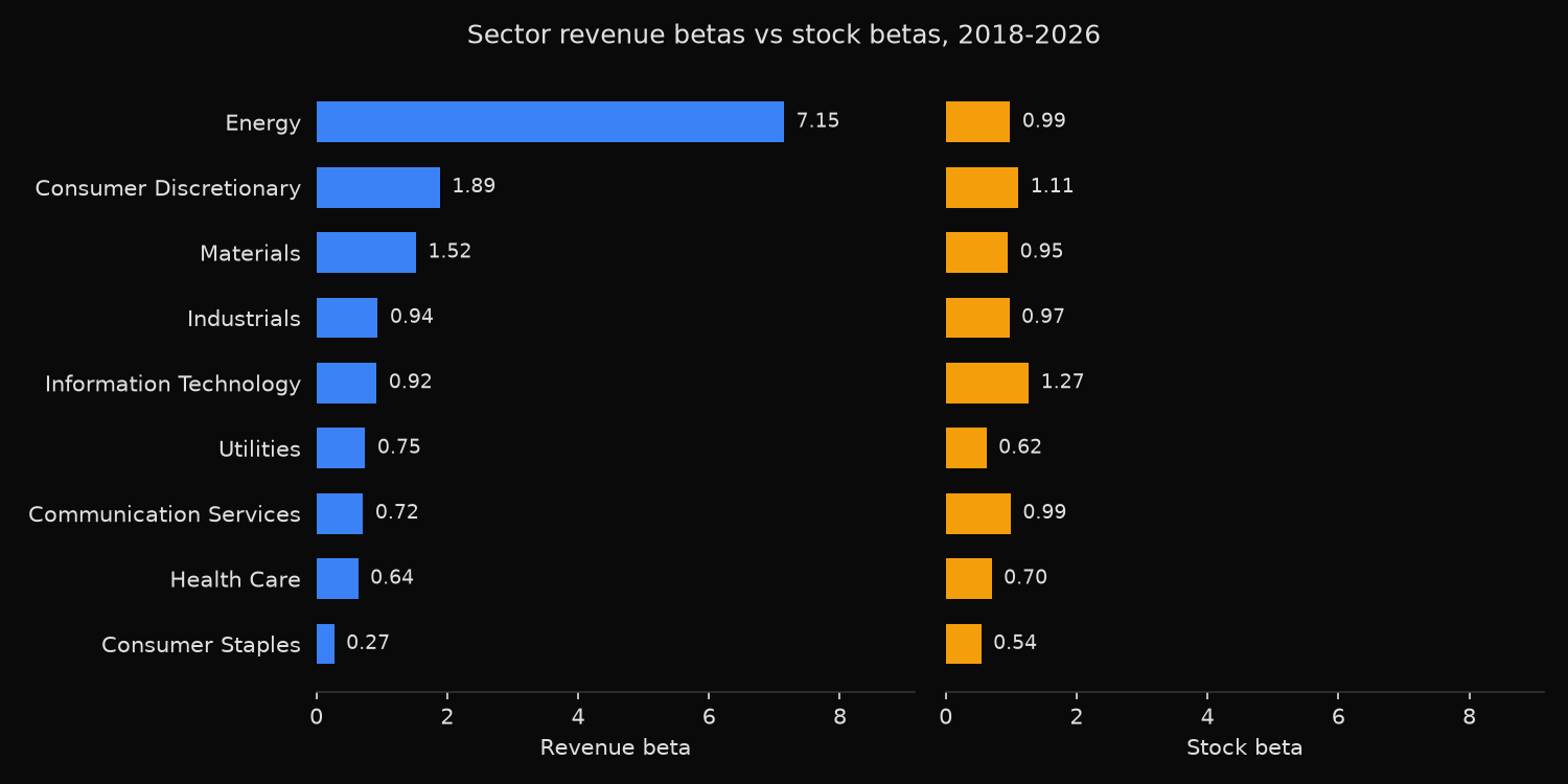
Firms per quarter: 367-397  quarters: 31  trading days: 1947
Corporate revenue cycle: trough -7.2% (2020Q2), peak +23.5% (2021Q2), latest +8.9%

Sector                   Rev beta      t     R2  ex-COVID  Stock beta  Worst qtr  Firms
Energy                       7.15    8.2   0.75      8.83        0.99    -55.0%     19
Consumer Discretionary       1.89    5.7   0.76      1.00        1.11    -28.7%     45
Materials                    1.52    6.7   0.74      2.29        0.95    -11.9%     23
Industrials                  0.94    6.8   0.71      0.63        0.97    -12.4%     70
Information Technology       0.92    9.3   0.63      1.39        1.27     -1.0%     55
Utilities                    0.75    3.2   0.29      1.50        0.62    -10.2%     28
Communication Services       0.72    6.5   0.57      0.61        0.99     -3.8%     17
Health Care                  0.64    3.8   0.54      0.28        0.70     -3.7%     54
Consumer Staples             0.27    4.9   0.40      0.36        0.54     -2.4%     27

Revenue beta range: 0.27 to 7.15 (26x)
Stock beta range:   0.54 to 1.27 (2.3x)
Rank correlation between the two: 0.53
What this tells us
Every sector has a positive revenue beta, with t-statistics from 3.2 to 9.3, measured against a cycle line that troughs at negative 7.2 percent in 2020Q2 and peaks at 23.5 percent in 2021Q2. The disagreement is about magnitude. Revenue betas span 0.27 to 7.15, a factor of 26; stock betas span 0.54 to 1.27, a factor of 2.3. The market compresses a very wide range of fundamental cyclicality into a narrow band around 1.
Energy is the clearest case. Its revenue swings roughly seven times the corporate cycle and median energy revenue fell 55 percent in 2020Q2, yet XLE carries a stock beta of 0.99. Energy revenue is price times volume, and the price is a commodity that moves far more than demand; the share prices a long strip of future oil prices, so one bad year of spot changes a modest fraction of the value.
Information Technology runs the mismatch in reverse, pairing the highest stock beta at 1.27 with a mid-table revenue beta of 0.92. Utilities are stranger: a revenue beta of 0.75 sits above Health Care and Communication Services against the second-lowest stock beta, because utility bills pass fuel costs through to customers. That estimate deserves the most caution, since its R-squared of 0.29 is the weakest in the table.
Dropping 2020Q2 through 2021Q2 leaves Energy at 8.83 and Consumer Staples at 0.36, so the spread is not a pandemic artefact. Two sectors do move. Consumer Discretionary halves to 1.00, meaning much of its measured cyclicality is the lockdown quarter, and Information Technology rises to 1.39.
So what?
The two betas answer different questions. Revenue beta is the input for scenario work on fundamentals: given a view on nominal corporate sales, it maps to what a sector’s top line does. Stock beta is the input for sizing the market risk of a position held today.
Substituting one for the other produces specific errors. Sizing an energy or materials position for a slowdown off a stock beta near 1 understates what happens to the earnings stream: the discount rate cushions the share price while the profit and loss takes the full hit. Buying technology as a bet on the economic cycle has the opposite problem, since those sales barely register the cycle.
Revenue is nominal, so both sides of every regression mix volume with price. For Energy that is the dominant effect and the reason its beta reaches 7.
The same comparison reruns on any grouping that matters to a given book, and point-in-time membership keeps survivorship out of the panel.
Built with xfinlink — free financial data API for Python.