
What’s the question?
A discounted cash flow model projects the cash a business will generate, discounts it back at a required rate of return, and returns one number for what the company is worth. Free cash flow here means cash from operations less capital expenditure.
The output looks like a measurement. It is not. Every input is a judgement about something nobody can observe: how fast cash flow grows, and what return an owner should demand for the risk of waiting. Two analysts reading the same filings and disagreeing only about whether to discount at 8% or 10% produce very different valuations, and neither can prove the other wrong.
A valuation model earns its place if it can say a price is wrong. If the range of fair values a careful analyst could defend is wide enough to swallow almost any market price, then the model reports the analyst’s priors rather than the company’s worth. This measures the width, across the current S&P 500.
The approach
Every company gets the same two-stage model: ten explicit years of free cash flow growth, then a terminal value growing forever at a constant rate, discounted at a single rate.
- Universe: current S&P 500 constituents, carried by permanent entity id. Financials and real estate leave the sample, because operating cash flow less capital expenditure does not describe those businesses.
- Base cash flow: the mean of the last three fiscal years, so one unusual year cannot set the valuation. Names whose three-year mean is not positive drop from the sample, which takes most of the utilities sector with it, since capital spending there routinely runs ahead of operating cash flow.
- Growth: each company’s own revenue growth rate compounded over six fiscal years, which keeps the 2020 trough out of the starting position. Floored at zero, capped at 12% a year.
- The grid: five discount rates from 7% to 11%, four terminal growth rates from 1.5% to 3.0%. Twenty valuations per company, every one of them defensible.
- Comparison: market capitalisation at that same fiscal year end, so price and cash flow describe the same moment.
Two assumptions sit outside the grid and are tested separately: the latest single year of free cash flow in place of the three-year mean, and fifteen explicit years in place of ten.
Code
import numpy as np
import pandas as pd
import xfinlink as xfl

xfl.set_api_key("YOUR_API_KEY")  # free at https://xfinlink.com/signup

RATES = [0.07, 0.08, 0.09, 0.10, 0.11]
TGROW = [0.015, 0.020, 0.025, 0.030]
YEARS, SPAN, G_CAP = 10, 6, 0.12

ids = sorted(int(i) for i in xfl.index("sp500")["entity_id"].dropna())
fun = xfl.fundamentals(entity_id=ids, period_type="annual",
                       start="2019-01-01", end="2026-06-30",
                       fields=["revenue", "free_cash_flow"], max_rows=60000)
cap = pd.concat([xfl.metrics(entity_id=ids[i:i + 60], period_type="annual",
                             start="2025-06-30", end="2026-06-30",
                             fields=["market_cap"], max_rows=20000)
                 for i in range(0, len(ids), 60)], ignore_index=True)

fun = fun[~fun["gics_sector"].isin(["Financials", "Real Estate"])]
rows = []
for eid, g in fun.sort_values("period_end").groupby("entity_id"):
    if len(g) < SPAN + 1 or g["period_end"].iloc[-1] < pd.Timestamp("2025-06-30"):
        continue
    fcf3 = g["free_cash_flow"].iloc[-3:]
    rev_now, rev_then = g["revenue"].iloc[-1], g["revenue"].iloc[-(SPAN + 1)]
    if fcf3.isna().any() or fcf3.mean() <= 0 or rev_then <= 0:
        continue
    rows.append({"entity_id": eid, "ticker": g["ticker"].iloc[-1],
                 "period_end": g["period_end"].iloc[-1], "base_fcf": float(fcf3.mean()),
                 "g1": float(np.clip((rev_now / rev_then) ** (1 / SPAN) - 1, 0.0, G_CAP))})

d = pd.DataFrame(rows).merge(cap[["entity_id", "period_end", "market_cap"]],
                             on=["entity_id", "period_end"], how="left")
d = d[d["market_cap"].between(1_000, 10_000_000)].reset_index(drop=True)

def dcf(fcf0, g1, r, gt, years=YEARS):
    yrs = np.arange(1, years + 1)
    cf = fcf0 * (1 + g1) ** yrs
    return float((cf / (1 + r) ** yrs).sum()
                 + cf[-1] * (1 + gt) / (r - gt) / (1 + r) ** years)

grid = [(r, gt) for r in RATES for gt in TGROW]
vals = np.array([[dcf(x.base_fcf, x.g1, r, gt) for r, gt in grid] for x in d.itertuples()])
d["v_min"], d["v_max"] = vals.min(axis=1), vals.max(axis=1)
d["band"] = d["v_max"] / d["v_min"]
d["pos"] = np.where(d["market_cap"] > d["v_max"], "above",
                    np.where(d["market_cap"] < d["v_min"], "below", "inside"))

print("median band %.2fx" % d["band"].median())
print(d["pos"].value_counts(normalize=True).mul(100).round(1).to_string())
Full script with formatting and visualisation: dcf-assumption-sensitivity-python.py
Output
A ten-year two-stage DCF over 5 discount rates x 4 terminal growth rates
Sample:    current S&P 500 ex financials and real estate; 329 companies clear the
           cash-flow and growth screens, 329 carry a market capitalisation on the
           same fiscal year end, 328 survive the sanity filter
Base:      mean free cash flow of the last 3 fiscal years, 2025-06-30 to 2026-06-30
Growth:    own 6-year revenue CAGR, floored at 0% and capped at 12%; median 6.0%

How wide is the answer?
  Highest / lowest fair value across the 20 cells
    median 2.26x      quartiles 2.19x to 2.39x      widest 2.42x
  Terminal value as a share of the central-cell value
    median 58.1%      quartiles 55.4% to 62.9%

Band width is a pure function of the growth assumed, not of the company
  Growth      1.0%   2.0%   4.0%   6.0%   8.0%  10.0%  12.0%
  Band width  2.11x   2.15x   2.20x   2.26x   2.32x   2.37x   2.42x
  TV share    52.2%   53.5%   55.9%   58.1%   60.2%   62.2%   64.0%

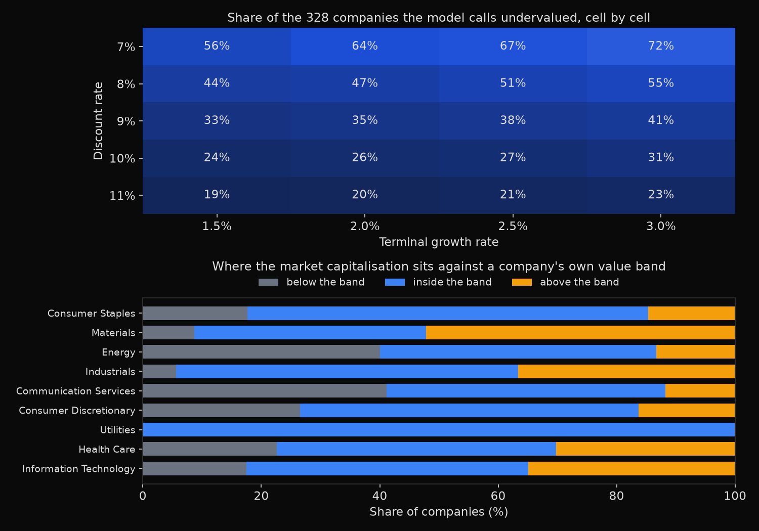
Share of the 328 companies the model calls undervalued, cell by cell
                          terminal growth
  Discount rate      1.5%     2.0%     2.5%     3.0%
          7.0%     55.8%    64.0%    66.8%    71.6%
          8.0%     44.2%    46.6%    50.6%    54.6%
          9.0%     32.6%    35.4%    38.1%    41.2%
         10.0%     24.1%    26.2%    27.4%    31.1%
         11.0%     18.6%    19.5%    21.0%    22.6%
  Same companies, same filings: 71.6% undervalued in the friendliest cell, 18.6% in the harshest

Can the model tell the market it is wrong?
  above the whole band    93   28.4%
  inside the band        174   53.0%
  below the whole band    61   18.6%
  market cap / central-cell value, median 1.18, quartiles 0.82 to 1.67

Two assumptions the grid never varies
  Base year: latest fiscal year free cash flow instead of the 3-year mean
    median absolute change 16.2%, upper quartile 33.5%, ninth decile 56.6%
    moves value further than the entire rate and terminal grid for 5 of 328 companies
  Horizon: 15 explicit years instead of 10
    median change +9.3%, quartiles +2.8% to +26.1%

By sector
                              n  growth     band  TV share    above   inside
  Consumer Staples           34    4.2%    2.21x     56.0%    14.7%    67.6%
  Materials                  23    4.4%    2.22x     56.4%    52.2%    39.1%
  Energy                     15    4.5%    2.22x     56.4%    13.3%    46.7%
  Industrials                71    5.3%    2.24x     57.3%    36.6%    57.7%
  Communication Services     17    5.7%    2.25x     57.7%    11.8%    47.1%
  Consumer Discretionary     49    6.4%    2.27x     58.5%    16.3%    57.1%
  Utilities                   3    7.3%    2.30x     59.4%     0.0%   100.0%
  Health Care                53    7.8%    2.31x     60.0%    30.2%    47.2%
  Information Technology     63    9.4%    2.35x     61.6%    34.9%    47.6%

The ten largest companies in the sample, $bn at their own fiscal year end
  Ticker  Year end     growth  base FCF  low value high value  market cap  verdict
  NVDA    2026-01-25    12.0%      61.5       1365       3299        4561    above
  GOOGL   2025-12-31    12.0%      71.8       1595       3852        3784   inside
  AAPL    2025-09-27     8.1%     102.4       1732       4018        3774   inside
  MSFT    2026-06-30    12.0%      70.9       1573       3801        2770   inside
  AMZN    2025-12-31    12.0%      24.3        539       1301        2477    above
  AVGO    2025-11-02    12.0%      21.3        473       1143        1752    above
  TSLA    2025-12-31    12.0%       4.7        105        253        1687    above
  META    2025-12-31    12.0%      48.1       1067       2578        1664   inside
  LLY     2025-12-31    12.0%       4.5        100        242        1014    above
  WMT     2026-01-31     5.2%      14.2        197        441         950    above
What this tells us
The band is 2.26x wide at the median and barely moves between companies: quartiles at 2.19x and 2.39x, nothing in the sample above 2.42x. A company growing at 1% a year gets 2.11x; one growing at 12% gets 2.42x. The imprecision is a property of discounting, not of what is being discounted.
What the grid does to the verdict is larger. At 7% and 3.0% terminal growth the model calls 71.6% of the sample undervalued; at 11% and 1.5%, the same model on the same filings calls 18.6% undervalued. That 53.0 point swing is, by construction, exactly the share of companies whose market capitalisation lands inside their own band.
For those 174 companies the model cannot say the price is wrong. The 93 above the most generous cell are the more interesting group, because no cell in the grid reaches their price. Tesla carries a three-year mean free cash flow of $4.7bn against a market capitalisation of $1,687bn, top of band $253bn; Lilly, $4.5bn against $1,014bn, top of band $242bn. Nvidia sits above its band too, and there the growth cap is talking rather than the company: revenue has compounded far faster than 12% a year and the model refuses to extrapolate it.
Terminal value carries 58.1% of the central-case valuation at the median and 64.0% for the fastest growers, so more than half the answer is a formula about 2036 onwards. The base year matters nearly as much: swapping the three-year mean for the latest single year moves value by 16.2% at the median, 56.6% at the ninth decile, and by more than the entire grid for 5 companies. That is an earnings-quality decision, not a market view.
So what?
Stop reporting a DCF as a number. A single fair value claims a precision the method does not have; the 2.26x band is the honest statement of what the model knows, with the assumptions producing each end printed beside it. A valuation that survives only at 7% and 3.0% is a view on the discount rate wearing a company’s name.
The productive direction is the reverse one. Solve for the growth rate that sets model value equal to today’s price, then judge whether that rate is achievable. "Priced for 12% growth for a decade" can be checked against a company’s own record; "fair value $312" cannot.
Give the base year the same scrutiny as the cost of equity. It is usually settled silently in one line of code, and it moves the answer by a third for a quarter of these companies. Before arguing about the discount rate, agree on which year’s cash flow is being grown.
Built with xfinlink — free financial data API for Python.