
How to Pick a Benchmark for a Backtest
September 16, 2026
A benchmark is honest when you could have bought it instead of running the strategy. Four things have to line up for that to hold: the universe the strategy selected from, the weighting scheme it applied, the return basis it is measured on, and the membership list as it stood on each date rather than as it stands today. Most disagreements about benchmarks are really disagreements about one of those four. The last is the expensive one, because a benchmark assembled from today’s index membership and run backwards is not a benchmark; it is a second strategy that knows the future.
Why Does the Benchmark Choice Change the Result?
Take one window, January 2017 to December 2025, and build three versions of “the S&P 500” from the same price file. The first is SPY, the cap-weighted proxy almost everyone reaches for. The second weights each member of the roster equally, refreshing membership every January from the roster as it actually stood at the prior year-end. The third weights equally as well, but uses the roster as it stands now and applies it to the whole period, which is what happens when a constituent list is downloaded once and reused.
import xfinlink as xfl
import pandas as pd

xfl.set_api_key("YOUR_API_KEY")  # free at https://xfinlink.com/signup

START, END = "2017-01-01", "2025-12-31"
YEARS = list(range(2017, 2026))

rosters = {y: xfl.index("sp500", as_of=f"{y - 1}-12-31") for y in YEARS}
today = xfl.index("sp500")
ids = sorted({int(i) for r in rosters.values() for i in r["entity_id"].dropna()}
             | {int(i) for i in today["entity_id"].dropna()})

frames = []
for i in range(0, len(ids), 100):
    frames.append(xfl.prices(entity_id=ids[i:i + 100], start=START, end=END,
                             interval="1mo", fields=["adj_close"], max_rows=200000))
px = pd.concat(frames, ignore_index=True)
px["month"] = px["date"].dt.to_period("M")
wide = px.pivot_table(index="month", columns="entity_id", values="adj_close")
ret = wide.pct_change()
ret = ret.drop(columns=ret.columns[(ret > 1.0).any()])

def equal_weight(members_by_year):
    return pd.Series({
        m: ret.loc[m, [c for c in members_by_year[m.year] if c in ret.columns]].dropna().mean()
        for m in ret.index[1:]
    })

pit = equal_weight({y: [int(i) for i in rosters[y]["entity_id"].dropna()] for y in YEARS})
now = equal_weight({y: [int(i) for i in today["entity_id"].dropna()] for y in YEARS})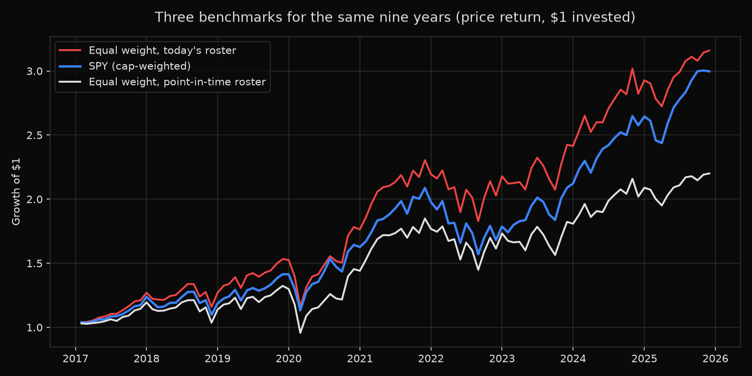
unique entities across 10 rosters: 677
priced entities: 674, excluded: 21, kept: 653
months: 2017-01 to 2025-12

benchmark                             growth     ann.      vol
SPY (cap-weighted)                     3.00x   13.10%   15.78%
Equal weight, point-in-time            2.20x    9.25%   17.41%
Equal weight, today's roster           3.16x   13.77%   16.92%

weighting choice (SPY - PIT equal weight): 3.85 pts/yr
survivorship gap (today's roster - PIT):   4.52 pts/yr
Returns here are price returns from adj_close, which is split-adjusted and does not include dividends. Names carrying a monthly move above 100% are excluded as suspected corporate-action artefacts, which removes 21 of 674 and makes the survivorship figure smaller rather than larger; without that screen the gap is 6.45 points a year.
Three benchmarks, one index, 4.52 points a year between the highest and the lowest. A strategy that compounded at 12% over this window beat the point-in-time equal-weight version by almost three points a year, lost to SPY by one, and lost to the contaminated construction by nearly two. Nothing about the strategy changed between those sentences.
Should the Benchmark Match the Universe or the Weighting?
Match the universe first, because it is the cheaper mistake to catch. A strategy that picks from S&P 500 members is not benchmarked by the Russell 2000, and a strategy holding forty mid-caps is not benchmarked by a large-cap index; the comparison mostly measures the size gap, and the strategy gets credit or blame for a decision it never made.
Weighting is the subtler half. If a strategy holds its positions in equal size, a cap-weighted benchmark asks a compound question: did the stock picks work, and was equal weighting the right call over this period? Those answers can point in opposite directions. Over 2017 to 2025 the weighting decision alone was worth 3.85 points a year, running in favour of cap weighting, which is roughly the size of the alpha most equity strategies claim. An equal-weighted strategy compared against SPY over these nine years is fighting a headwind that belongs to the benchmark rather than to its own stock selection. Report against both and the source of the difference stops being ambiguous.
Does the Benchmark Need Point-in-Time Membership?
If you take a published index level, the point-in-time work is already done for you; index providers do not retroactively rewrite membership. The problem appears the moment you build a benchmark yourself, which is normal whenever the strategy trades a universe no published index matches, or whenever the fair comparison is an equal-weighted version of an index that is published cap-weighted.
The output above puts a number on it. The same equal-weight rule, over the same months, with the same price file, returns 9.25% a year on the roster as it stood and 13.77% on the roster as it stands now. That 4.52-point gap is pure look-back: today’s list contains companies that were added after they had already run, and omits every member that was acquired, delisted or removed for underperformance. A benchmark carrying that bias is a benchmark almost nothing beats, which is the failure mode that quietly kills strategies before they reach production. The mechanism is set out further in what is survivorship bias in backtesting.
Building the honest version needs two things that are easy to state and awkward to source: a roster dated to each rebalance, and an identifier that survives ticker changes so the roster joins to the right price series. In xfinlink, index("sp500", as_of="2019-12-31") returns membership on that date with the ticker and company name each member carried then, and entity_id is the stable key that joins those rows to prices() even when the symbol later changed hands. Membership events go back to 1957 for the S&P 500, 1979 for the Russell 2000 and 1995 for the Nasdaq 100, and the same as_of parameter works on all of them.
Price Return or Total Return?
Both sides of the comparison must sit on the same basis, and the gap between the two bases is large enough to decide a result on its own. Yahoo Finance publishes the S&P 500 price index under ^GSPC, which closed at 7,585.73 on 15 September 2026, and the total-return version under ^SP500TR, which closed at 17,007.90 the same day (finance.yahoo.com, as of September 2026). Those two series describe the same 500 companies. The difference between them is dividend reinvestment.
Pick either basis and hold it on both sides. The figures above are price returns on both the strategy side and the benchmark side, which is internally consistent; comparing a dividend-inclusive strategy against ^GSPC is not, and it credits the strategy with roughly the index yield every year. The xfinlink field documentation states plainly that adj_close is adjusted for splits and not for dividends, so there is no ambiguity about which basis a column is on. What that adjustment does and does not cover is set out in split adjustment explained.
Where Do You Get the Benchmark Series?
| Source | What it gives you | Checked |
|---|---|---|
| Yahoo Finance index symbols | ^GSPC price level and ^SP500TR total-return level, free on the quote pages | finance.yahoo.com, September 2026 |
| yfinance | An unofficial Python client for Yahoo’s public APIs. Its README states the project is “not affiliated, endorsed, or vetted by Yahoo, Inc.”, is “intended for research and educational purposes”, and that “the Yahoo! finance API is intended for personal use only” | github.com/ranaroussi/yfinance, September 2026 |
| Alpha Vantage | Index Data endpoints covering S&P 500 (SPX), Dow Jones (DJI), Nasdaq Composite (COMP), Nasdaq-100 (NDX), Russell 2000 and the VIX, with daily, weekly and monthly OHLC | alphavantage.co/documentation, September 2026 |
| Kenneth French Data Library | The US market excess return series (Mkt-RF) in daily, weekly and monthly files, data through July 2026 | mba.tuck.dartmouth.edu, September 2026 |
| xfinlink | ETF and stock prices, plus point-in-time index rosters through index(as_of=) and a stable entity_id for joining them | xfinlink.com/docs |
For a single line on a chart, a published level is the shortest path, and Alpha Vantage serving index OHLC directly is genuinely convenient. A level series answers the question of what the index did. It does not answer the question of who was in it, and that second question is the one that decides whether a benchmark you construct yourself is measuring the strategy or flattering it.
FAQ
Is SPY an acceptable stand-in for the S&P 500? For most work, yes. An ETF price reflects fund expenses, cash drag and its own dividend treatment, while a published index level does not, so the two diverge slowly. Decide which basis the strategy is on before choosing between them.
Should a backtest report more than one benchmark? Reporting against a cap-weighted and an equal-weighted version of the same universe costs one extra column and separates stock selection from the weighting decision. The gap between them over 2017 to 2025 was 3.85 points a year, which is too large to leave unattributed.
What if the strategy trades a universe with no published index? Build the benchmark from the same selection rule with equal weights, sourcing membership point-in-time at each rebalance date. That construction has no look-ahead in it, which the roster you download today does.
pip install -U xfinlink