How Many Independent Bets Does a Nine-Sector Portfolio Give You? Eigenvalue Analysis in Python

July 29, 2026

What’s the question?

Nine sector funds look like nine positions. They rarely behave like nine. When every sector moves together, the account holds one position bought nine times, and a risk report listing nine line items is describing bookkeeping rather than risk.

The quantity that matters is the effective number of independent bets. Extract the eigenvalues of the correlation matrix of the nine daily return series. Each one measures how much variance sits along an uncorrelated direction, and the nine always sum to nine. Perfect independence puts one unit in each direction; perfect co-movement piles all nine into the first. Collapsing that spread into a single figure uses the entropy of the normalised eigenvalues, exponentiated:

N = exp(-sum(p_i * ln p_i)),   p_i = lambda_i / 9

N lands on the same scale as the position count, so it reads without translation. Nine means nine genuine bets. Two means two. Two questions follow: how far below nine does a standard sector allocation sit, and what does the shortfall cost in volatility?

The approach

The universe is the nine original Select Sector SPDR funds, which partition the S&P 500 and have traded since December 1998. Real estate and communication services, added later, are left out so that one cross-section runs across the whole 27 years.

1. Pull daily adj_close from December 1998 to 24 July 2026. It is split-adjusted and gap-free, which matters: five of these funds split two-for-one on 5 December 2025, and a raw quoted price would enter the sample as a 50% single-day loss.
2. Convert to daily returns, keeping the dates every fund trades so all nine correlations rest on the same observations.
3. On each trailing 252-day window, build the 9x9 correlation matrix, take its eigenvalues, and convert them to N.
4. Measure the realised benefit over the same window: volatility of the equal-weight blend against the average volatility of its nine parts.
5. Read the series at five stress episodes and at the most recent window.

Two checks guard the arithmetic. Eigenvalues of a correlation matrix must sum to the number of assets, and every one of the 6,680 windows returns 9.000000. An entropy measure is also only worth computing if it tracks something an investor can spend; N moves with the realised volatility reduction at 0.988.

Code

import numpy as np
import pandas as pd
import xfinlink as xfl

xfl.set_api_key("YOUR_API_KEY")  # free at https://xfinlink.com/signup

SECTORS = ["XLB", "XLE", "XLF", "XLI", "XLK", "XLP", "XLU", "XLV", "XLY"]
WINDOW = 252

frames = [xfl.prices(t, start="1998-12-01", end="2026-07-24",
                     fields=["adj_close"], max_rows=20000) for t in SECTORS]
px = pd.concat(frames).pivot(index="date", columns="ticker", values="adj_close").dropna()
rets = px.pct_change().dropna()

n = rets.shape[1]
R = rets.values
rows = []
for i in range(WINDOW - 1, len(rets)):
    corr = np.corrcoef(R[i - WINDOW + 1:i + 1], rowvar=False)
    eig = np.sort(np.linalg.eigvalsh(corr))[::-1]
    p = np.clip(eig / n, 1e-12, None)
    rows.append((rets.index[i],
                 float(np.exp(-(p * np.log(p)).sum())),
                 eig[0] / n,
                 corr[np.triu_indices(n, 1)].mean()))

res = pd.DataFrame(rows, columns=["date", "n_eff", "pc1", "avg_corr"]).set_index("date")

sector_vol = rets.rolling(WINDOW).std().mean(axis=1)
port_vol = rets.mean(axis=1).rolling(WINDOW).std()
res["vol_cut"] = (1 - port_vol / sector_vol).reindex(res.index)

print(res.loc[["2012-06-29", "2020-03-31", res.index[-1]]])
print("N vs realised volatility reduction:", round(res["n_eff"].corr(res["vol_cut"]), 3))

Full script with formatting and visualisation: sector-diversification-effective-bets-pca-python.py

Output

Nine Select Sector SPDR funds, daily price returns from split-adjusted closes
Sample      : 1998-12-23 to 2026-07-24 (6,931 trading days, 6,680 rolling windows)
Window      : 252 trading days
Check       : eigenvalues sum to 9.000000 - 9.000000 (must equal 9)

EFFECTIVE NUMBER OF INDEPENDENT BETS   (maximum possible = 9)
                            window end      N   PC1 share  avg corr  vol cut  port vol
Dot-com unwind              2002-09-30   3.58       67.2%      0.62    18.1%     22.7%
Global financial crisis     2008-11-28   2.75       75.6%      0.72    13.2%     36.1%
Euro sovereign crisis       2012-06-29   1.80       87.8%      0.86     5.8%     23.1%
COVID crash                 2020-03-31   1.90       85.7%      0.84     7.7%     30.6%
Inflation shock             2022-09-30   3.47       65.7%      0.59    20.9%     18.8%
Latest window               2026-07-24   6.33       36.6%      0.23    44.6%      9.6%

WHAT A GIVEN N IS WORTH
     N range   windows   avg corr   volatility removed
   below 2.5       887       0.82                 8.2%
   2.5 - 3.0     1,046       0.71                13.5%
   3.0 - 3.5     1,372       0.64                17.5%
   3.5 - 4.0     1,550       0.57                21.8%
   4.0 - 4.5       649       0.51                25.5%
   above 4.5     1,176       0.38                33.2%

Window sensitivity: April 2025 on its own carries an average pairwise correlation of 0.85 across 21 days.
  252 days to 2026-03-31            N = 4.14
  same window minus April 2025      N = 5.73

Full-sample low  : 1.80 on 2012-06-29   high: 6.42 on 2001-03-19   median: 3.53
Latest reading   : 6.33, above 99.6% of all windows since 1999
N tracks the realised volatility reduction with a correlation of 0.988

What this tells us

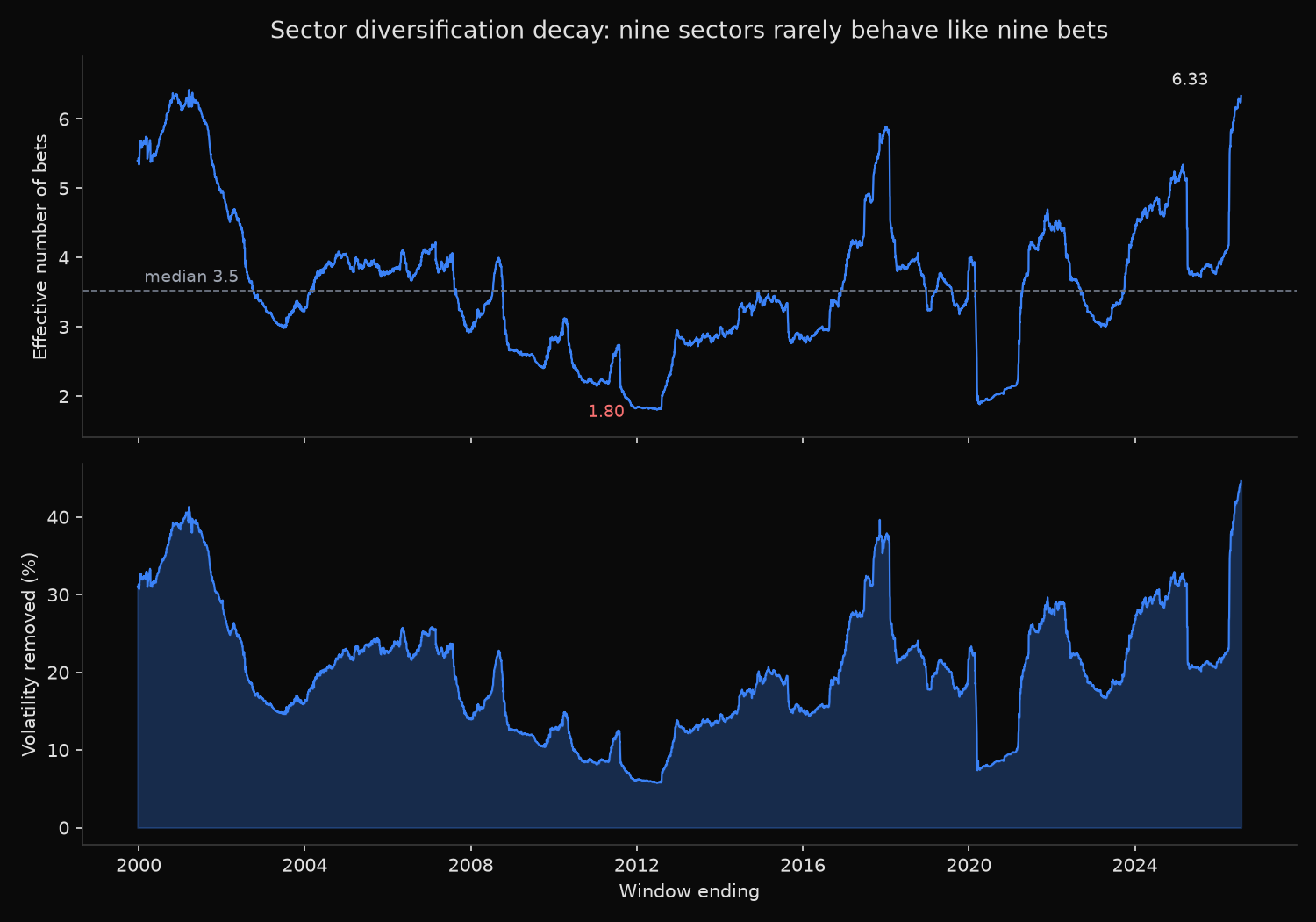
Nine sectors have never once delivered nine bets. The median window returns 3.53, so a fully spread sector sleeve behaves like three and a half independent positions on an ordinary day.

The collapse is worst where it hurts. At the euro sovereign crisis trough in June 2012, N reached 1.80, the first principal component absorbed 87.8% of variance, and average pairwise correlation stood at 0.86. Holding all nine sectors removed 5.8% of the volatility of holding one average sector: nine positions, a 6% risk reduction. The COVID window ending March 2020 is close behind at 1.90, and 2008 is milder than either at 2.75. The deepest crash was not the worst diversification failure. The 2011 to 2012 risk-on, risk-off regime was, which lines up with the record highs in option-implied index correlation printed over the same stretch.

The bucket table puts a price on it. Below N = 2.5, an equal-weight blend strips out 8.2% of average single-sector volatility; above N = 4.5, it strips out 33.2%. Same nine holdings, four times the benefit.

The latest window is an outlier: N reads 6.33, average pairwise correlation sits at 0.23, and the blend removes 44.6% of single-sector volatility. Only 24 earlier days out of 6,680 scored higher, all in the dispersion regime of 2000 and 2001.

A rolling estimate is hostage to what sits inside the window. April 2025 carried an average pairwise correlation of 0.85 across 21 trading days and dominated every window containing it: the 252 days to 31 March 2026 read 4.14 with that month in and 5.73 without it. Most of the jump through April 2026 is one shock month ageing out.

So what?

Size risk against N rather than against the position count. A nine-sector sleeve run to a volatility target should carry a smaller notional when N sits near 2 than when it sits near 5, because the identical holdings deliver an 8% volatility reduction in the first case and 33% in the second. A rebalancing rule built on a fixed assumed correlation levers up precisely when correlation spikes.

Treat N as a state variable, not a forecast. Computed from trailing data, it says nothing about direction. It answers the question a position report cannot: whether the diversification a mandate is credited with currently exists.

Right now it does. Sector dispersion has not been this wide since 2001. That is a regime rather than a constant, and the 1.80 of June 2012 is what these same nine funds look like when the regime ends.