What Actually Drives Return on Equity? DuPont Decomposition in Python

August 17, 2026

What’s the question?

Return on equity is the number most investors reach for when they want one measure of how well a company converts shareholder capital into profit. It is net income divided by book equity. Two companies can both report 20 percent and be nothing alike: one sells a rare product at a high price, another sells an ordinary product very quickly, and a third gets there by financing its assets with debt rather than equity.

The DuPont identity separates those cases. It rewrites return on equity as the product of three ratios:

net income / equity = (net income / revenue) x (revenue / assets) x (assets / equity)

The first term is net profit margin, the profit kept from each dollar of sales. The second is asset turnover, the revenue produced by each dollar of assets, which measures how hard the asset base works. The third is the equity multiplier, assets divided by book equity, which rises as a company funds itself with more debt and less equity. Revenue and assets cancel, so the identity is arithmetic rather than a model, and it holds exactly for every company.

That leaves an empirical question the identity itself cannot answer. Across a large universe of companies, which of the three parts explains why some earn 40 percent on equity and others earn 4 percent? If the answer is leverage, a high return on equity says more about the financing decision than about the business. If the answer is margin, it points to pricing power and cost discipline.

The approach

The sample is the current S&P 500, measured over fiscal years ending in calendar 2024. Members are identified by their permanent entity id rather than by ticker symbol, so a company that has changed symbol is still matched to its own financials.

1. Pull revenue, net income, total assets and total equity for every member.
2. Keep the fiscal year ending inside calendar 2024, so each company contributes one comparable twelve-month period.
3. Compute the three components and return on equity directly from those four line items, which makes the identity exact to machine precision rather than approximate.
4. Keep companies with positive net income, positive revenue, and book equity of at least 1 percent of total assets. Logarithms require positive values, and an equity base near zero sends the ratio toward infinity without revealing anything about the underlying business. This leaves 443 companies out of 499.
5. Take logarithms. Since log ROE is the sum of the three log components, the cross-sectional variance of log ROE splits exactly into three parts: each component’s share is its covariance with log ROE divided by the variance of log ROE, and the shares sum to 100 percent.

The covariance form is what makes the decomposition meaningful. A component that varies wildly can still contribute almost nothing if its variation is unrelated to return on equity, or if it moves in a way that cancels another component. Sorting companies by leverage alone would not reveal that.

Code

import numpy as np
import pandas as pd
import xfinlink as xfl

xfl.set_api_key("YOUR_API_KEY")  # free at https://xfinlink.com/signup

members = xfl.index("sp500")
ids = members["entity_id"].dropna().astype(int).tolist()

frames = []
for i in range(0, len(ids), 100):
    frames.append(xfl.fundamentals(
        entity_id=ids[i:i + 100], period_type="annual", start="2024-01-01", end="2025-06-30",
        fields=["revenue", "net_income", "total_assets", "total_equity", "gics_sector"]))
f = pd.concat(frames, ignore_index=True)
f["period_end"] = pd.to_datetime(f["period_end"])
f = f[(f["period_end"] >= "2024-01-01") & (f["period_end"] <= "2024-12-31")]

f["margin"] = f["net_income"] / f["revenue"]
f["turnover"] = f["revenue"] / f["total_assets"]
f["leverage"] = f["total_assets"] / f["total_equity"]
f["roe"] = f["net_income"] / f["total_equity"]

d = f.dropna(subset=["margin", "turnover", "leverage", "roe", "gics_sector"])
pos = d[(d["net_income"] > 0) & (d["revenue"] > 0)
        & (d["total_equity"] / d["total_assets"] >= 0.01)].copy()
for src, dst in [("margin", "lm"), ("turnover", "lt"), ("leverage", "ll"), ("roe", "lr")]:
    pos[dst] = np.log(pos[src])


def decompose(frame, label):
    var = frame["lr"].var(ddof=1)
    print(f"
{label}  n={len(frame)}  sd(log ROE)={np.sqrt(var):.3f}")
    for col, name in [("lm", "Net margin"), ("lt", "Asset turnover"), ("ll", "Equity multiplier")]:
        print(f"  {name:<18} {frame[col].cov(frame['lr']) / var * 100:5.1f}%")


decompose(pos, "All sectors")
decompose(pos[~pos["gics_sector"].isin(["Financials", "Real Estate", "Utilities"])],
          "Operating companies only")
decompose(pos[pos["gics_sector"] == "Financials"], "Financials only")

Full script with formatting and visualisation: dupont-roe-decomposition-sp500-python.py

Output

All sectors  n=443  sd(log ROE)=1.014
  Net margin          38.2%
  Asset turnover      32.5%
  Equity multiplier   29.3%

Operating companies only  n=313  sd(log ROE)=1.029
  Net margin          45.4%
  Asset turnover      17.9%
  Equity multiplier   36.7%

Financials only  n=72  sd(log ROE)=0.671
  Net margin          34.6%
  Asset turnover      55.4%
  Equity multiplier   10.0%

Sector medians, fiscal 2024
                         n    roe  margin  turnover  leverage
gics_sector
Consumer Discretionary  39  0.333   0.093     1.006     2.936
Industrials             72  0.252   0.128     0.754     2.628
Information Technology  60  0.226   0.178     0.512     2.067
Consumer Staples        33  0.177   0.082     0.865     2.637
Communication Services  15  0.176   0.130     0.466     2.167
Materials               26  0.163   0.096     0.643     2.432
Energy                  21  0.152   0.123     0.522     2.316
Financials              72  0.143   0.203     0.186     5.249
Health Care             47  0.129   0.118     0.548     2.175
Utilities               30  0.094   0.144     0.190     3.823
Real Estate             28  0.060   0.168     0.142     2.011

What this tells us

Across the full sample no single component dominates. Margin carries 38.2 percent of the spread in log return on equity, asset turnover 32.5 percent, and the equity multiplier 29.3 percent. Anyone expecting leverage to account for most of the difference between a high-ROE company and a low-ROE one is wrong at the index level.

Splitting the sample by business type produces two very different pictures. Among operating companies, meaning everything outside financials, real estate and utilities, margin carries 45.4 percent and turnover only 17.9 percent. Industrial and consumer businesses run asset bases of broadly similar intensity, so what separates them is how much profit survives the journey from revenue to net income.

Financials invert this completely. The equity multiplier explains 10.0 percent of the spread among banks and insurers, the smallest share anywhere in the study, even though financials are by far the most levered sector with a median multiplier of 5.25 against roughly 2.3 elsewhere. High leverage is universal in that sector rather than distinguishing, and capital regulation compresses the range further. What separates a profitable financial institution from an unprofitable one is asset turnover, at 55.4 percent of the spread: revenue generated per dollar of balance sheet.

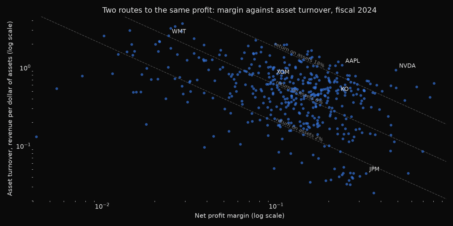
The sector medians show both routes to a good return. Consumer Discretionary posts the highest median return on equity at 33.3 percent on a slim 9.3 percent margin, because its assets turn over roughly once a year. Information Technology reaches 22.6 percent from the opposite direction, with a 17.8 percent margin and turnover of just 0.51. Real Estate sits at the bottom on 6.0 percent despite a 16.8 percent margin, held back by turnover of 0.14. Fat margins on a slow asset base do not produce a good return on capital.

The chart makes the trade-off visible. Companies cluster along the dashed curves of constant return on assets, with Walmart at a 2.4 percent margin turning its assets 2.55 times a year and Nvidia at a 48.9 percent margin turning them 0.93 times. Both are excellent businesses, and they are excellent in incompatible ways.

So what?

A screen that ranks companies by return on equity should not be used on its own, because it mixes three unrelated qualities into a single number. Run the decomposition alongside it. For an operating company, check whether a high figure comes from margin, which tends to persist, or from an equity multiplier far above the sector median, which is a financing choice that can be reversed and that deepens the damage a downturn does.

For banks and insurers, comparing leverage is close to useless. It is nearly constant within the sector and explains almost nothing about which institution earns more. Revenue per dollar of assets is the number that separates them.

The same decomposition applied to a single company across ten years answers a harder and more useful question: when return on equity improved, did the business get better at converting sales into profit, or did the balance sheet simply get thinner? Only the first kind of improvement deserves a higher multiple.

Built with xfinlink — free financial data API for Python. pip install -U xfinlink