
What’s the question?
Idiosyncratic volatility is what remains of a stock’s daily movement once the market’s movement is taken out. Fit the stock’s returns on the market’s, keep the residuals, take their standard deviation, and the result measures how much the stock moves for reasons of its own.
Textbook asset pricing says that number should have nothing to do with expected return, because company-specific risk can be diversified away and nobody is paid for carrying what they could shed for free. Ang, Hodrick, Xing and Zhang reported the opposite in 2006, and worse than the opposite: the highest idiosyncratic volatility went with the lowest subsequent returns.
Two things decide whether a fresh test of that means anything. The spread needs a t-statistic, because a long-short return of a few tenths of a percent a month looks like a strategy and is usually noise. And residual volatility has to be told apart from plain volatility, since a residual sort that merely reproduces a volatility sort has found nothing new. A quintile sort on total volatility carries out the plain version on the same index.
The approach
The sample is the S&P 500 as it actually stood at 119 month ends between February 2016 and December 2025, from point-in-time rosters covering 713 companies. Names are carried by entity id, so a recycled or changed ticker does not swap one company for another mid-test.
- At each month end, take that month’s roster and the daily price returns from split-adjusted closes over the 252 trading days ending on the sort date. Names with fewer than 240 observations there, or a gap in the holding month, drop from that sort.
- Fit those returns on SPY daily returns by ordinary least squares over the same window. Idiosyncratic volatility is the annualised standard deviation of the residuals; total volatility that of the raw returns.
- Sort into quintiles on each measure separately, hold equal-weighted for a month, record quintile 5 minus quintile 1.
- Double sort to separate the two: inside each total-volatility quintile, split on idiosyncratic volatility into terciles, take high minus low, average across the five.
Daily moves above +100% or below -50% mark corporate actions rather than returns, and the 30 names carrying one leave the sample. Returns are price returns; low-volatility names carry the higher dividend yields, so this works against the hypothesis rather than for it.
Code
import numpy as np
import pandas as pd
import xfinlink as xfl
from concurrent.futures import ThreadPoolExecutor

xfl.set_api_key("YOUR_API_KEY")  # free at https://xfinlink.com/signup

months = pd.date_range("2015-01-31", "2025-12-31", freq="ME")
roster = {d: xfl.index("sp500", as_of=d.strftime("%Y-%m-%d"))["entity_id"].tolist()
          for d in months}
ids = sorted({e for v in roster.values() for e in v})
chunks = [ids[i:i + 90] for i in range(0, len(ids), 90)]

grab = lambda cy: xfl.prices(entity_id=cy[0], start=f"{cy[1]}-01-01", end=f"{cy[1]}-12-31",
                             fields=["adj_close"], max_rows=60000)
with ThreadPoolExecutor(4) as ex:
    px = pd.concat(ex.map(grab, [(c, y) for y in range(2015, 2026) for c in chunks]))
spy = xfl.prices("SPY", start="2015-01-01", end="2025-12-31", fields=["adj_close"])

mkt = spy.set_index("date")["adj_close"].sort_index()
P = px.drop_duplicates(["entity_id", "date"]).pivot(index="date", columns="entity_id",
                                                    values="adj_close")
R = P.sort_index().reindex(mkt.index).pct_change()
R = R.drop(columns=R.columns[((R > 1.0) | (R < -0.5)).any()])  # corporate-action artefacts
M, col = mkt.pct_change().values, {c: i for i, c in enumerate(R.columns)}

sd = [(d, R.index.searchsorted(d, "right") - 1) for d in months]
sd = [(d, p) for d, p in sd if p >= 252 and R.index[p].to_period("M") == d.to_period("M")]
rank = lambda x, q: np.argsort(np.argsort(x)) * q // len(x)

recs = []
for (d, p), (_, nxt) in zip(sd[:-1], sd[1:]):
    j = [col[e] for e in roster[d] if e in col]
    W, F, m = R.values[p - 251:p + 1, j], R.values[p + 1:nxt + 1, j], M[p - 251:p + 1]
    ok = ((~np.isnan(W)).sum(0) >= 240) & ((~np.isnan(F)).sum(0) == F.shape[0])
    W, F = np.nan_to_num(W[:, ok]), F[:, ok]
    md = m - m.mean()
    beta = (W - W.mean(0)).T @ md / (md @ md)
    resid = W - (W.mean(0) - beta * m.mean()) - np.outer(m, beta)
    recs.append((resid.std(0, ddof=2) * np.sqrt(252), W.std(0, ddof=1) * np.sqrt(252),
                 np.prod(1 + F, axis=0) - 1))

t = lambda x: x.mean() / (x.std(ddof=1) / np.sqrt(len(x)))
for k, label in ((0, "Idiosyncratic vol"), (1, "Total vol")):
    q = np.array([[f[rank(v[k], 5) == i].mean() for i in range(5)] for *v, f in recs])
    s = q[:, 4] - q[:, 0]
    print(f"{label:<18}" + "".join(f"{x*100:7.2f}%" for x in q.mean(0)) +
          f"   5-1 {s.mean()*100:5.2f}%   t {t(s):5.2f}")

cond = np.array([np.mean([f[g][rank(iv[g], 3) == 2].mean() - f[g][rank(iv[g], 3) == 0].mean()
                          for g in [rank(tv, 5) == i for i in range(5)]])
                 for iv, tv, f in recs])
print(f"{len(recs)} months. Idiosyncratic vol high minus low, holding total vol fixed: "
      f"{cond.mean()*100:.2f}% a month, t {t(cond):.2f}")
Full script with formatting and visualisation: idiosyncratic-volatility-puzzle-sp500-python.py
Output
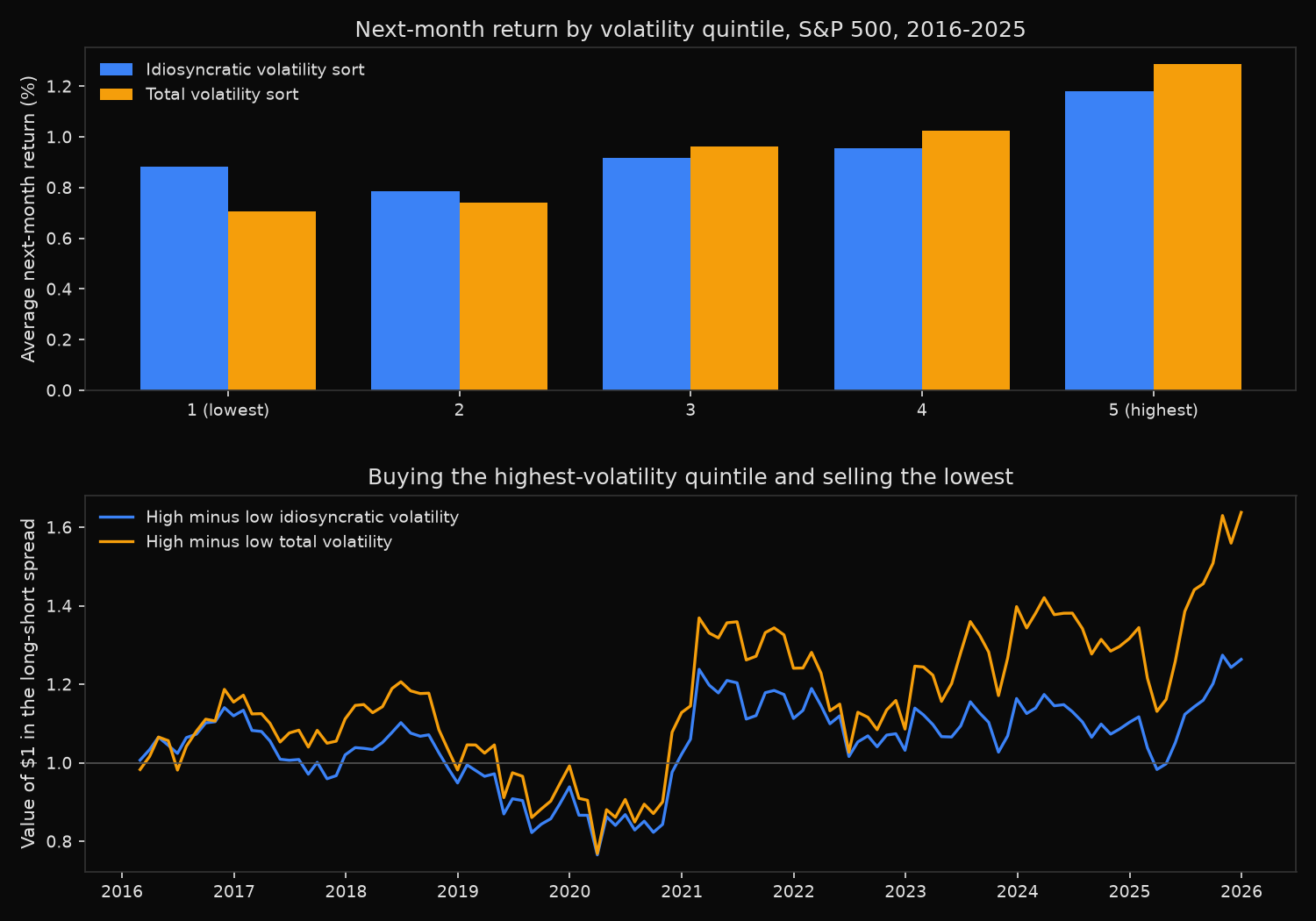
Idiosyncratic volatility and next-month returns, point-in-time S&P 500
Panel:    119 monthly sorts, 2016-02 to 2025-12; 713 companies appear on a roster,
          30 drop on the daily-return screen; median 482 names ranked per sort (range 469 to 486)
Formation: 252 trading days of daily price returns, market model against SPY
Holding:  equal-weighted, one month, no skip

Average next-month return by quintile (1 = lowest volatility, 5 = highest)
  Quintile              1       2       3       4       5    5 minus 1        t
  Idiosyncratic vol    0.88%   0.79%   0.92%   0.95%   1.18%       0.30%     0.71
  Total vol            0.71%   0.74%   0.96%   1.02%   1.29%       0.58%     1.09

  Average annualised volatility in each quintile
  Idiosyncratic vol    16.1%   19.6%   22.8%   27.2%   39.3%
  Total vol            20.3%   24.6%   28.4%   33.4%   46.0%

Annualised long-short return (quintile 5 minus quintile 1)
  Idiosyncratic vol     3.64%   monthly   0.30%   t =  0.71   hit rate 53.8%
  Total vol             7.19%   monthly   0.58%   t =  1.09   hit rate 56.3%

Are the two sorts the same sort?
  Cross-sectional rank correlation, idiosyncratic vs total vol   0.915 (0.751 to 0.981)
  Top quintile shared by both rankings                           86.6%
  Rank correlation of idiosyncratic vol with market beta         0.428
  Correlation of the two monthly long-short return series        0.965

How wide is the uncertainty on the monthly long-short return?
  Idiosyncratic vol   0.30%   standard error 0.42%   95% interval  -0.53% to  1.13%
  Total vol           0.58%   standard error 0.53%   95% interval  -0.47% to  1.63%

Holding for a quarter instead of a month, non-overlapping
  Idiosyncratic vol 39 quarters   quintile 5 minus 1   0.88%   t =  0.72
  Total vol         39 quarters   quintile 5 minus 1   1.81%   t =  1.18

Double sort: hold one dimension fixed, sort on the other
  Idiosyncratic vol high minus low, within total-vol quintiles    -0.14% a month   t = -0.79
  Total vol high minus low, within idiosyncratic-vol quintiles     0.54% a month   t =  1.67

  Idiosyncratic-vol spread inside each total-vol quintile
  Total-vol quintile    1       2       3       4       5
  High minus low    -0.21%  -0.07%  -0.33%  -0.30%   0.21%

Long-short return by calendar year (quintile 5 minus quintile 1)
  Year    Idio vol   Total vol
  2016      11.98%      15.48%
  2017      -8.89%      -3.73%
  2018      -7.01%     -11.69%
  2019      -1.04%       1.05%
  2020       8.86%      13.70%
  2021       8.90%      10.01%
  2022      -7.29%     -12.50%
  2023      12.78%      28.73%
  2024      -5.22%      -5.82%
  2025      14.54%      24.40%
What this tells us
The puzzle does not appear here. Average next-month returns climb with idiosyncratic volatility rather than falling: 0.88%, 0.79%, 0.92%, 0.95%, 1.18% across the quintiles, the noisiest names paying 0.30% a month more than the calmest, or 3.64% a year. That is the opposite sign to the one Ang, Hodrick, Xing and Zhang reported.
The number is also not evidence of anything. Standard error 0.42% a month, t-statistic 0.71, 95% interval running from -0.53% to +1.13%. Ten years of monthly sorts on roughly 482 names cannot tell a large negative premium apart from a large positive one. A quarterly holding period gives the same verdict at t = 0.72, and the spread lost money in five of the ten calendar years.
The second question has a much sharper answer. Sorting on idiosyncratic volatility is very nearly the same act as sorting on total volatility: rank correlation between the two averages 0.915, 86.6% of the top quintile is shared, and the two monthly long-short return series correlate 0.965. Residualising strips out the market component, a modest share of daily variance for a typical S&P 500 name, so the ordering barely moves.
Hold total volatility fixed and the residue changes sign. Idiosyncratic volatility inside total-volatility quintiles pays -0.14% a month at t = -0.79, negative in four of the five. The original paper’s direction survives as a small tilt inside a volatility sort rather than as an effect standing on its own, and it is still indistinguishable from zero. Reverse the roles and total volatility inside idiosyncratic-volatility quintiles pays 0.54% at t = 1.67.
So what?
Do not put money behind either spread. Neither clears conventional significance at either horizon, and an interval spanning -0.53% to +1.13% a month is not a signal; it measures how little a decade of monthly sorts settles.
The result that does travel is the correlation. Before adding a residualised version of any signal to a book that already holds the raw version, measure the rank correlation of the two scores and the correlation of the two long-short return series. Here they are 0.915 and 0.965. A covariance matrix built from those two streams will report a diversification benefit that does not exist, and a risk model carrying both will double-count one exposure under two labels. Anyone testing the anomaly itself should read the double sort as the design brief: neutralise total volatility from the start rather than in an appendix.
Built with xfinlink — free financial data API for Python.