Does a Bollinger Band Squeeze Predict a Big Move? Band Width Analysis in Python

September 13, 2026

What’s the question?

Bollinger Bands place two lines around a 20-day moving average of price, each two standard deviations away. The gap between them, divided by the average, is band width: a measure of how far the stock has travelled over the past month. When band width falls to the bottom of its own recent range, charting software calls it a squeeze, and the conventional reading is that a large move is coming.

Two claims hide inside that reading and are rarely separated. The first is that volatility mean-reverts, so an unusually calm month tends to be followed by a less calm one. The second is that a squeeze precedes a big move in absolute terms: the next month is wilder than a typical month, not merely wilder than the quiet one before it. A breakout buyer is relying on the second claim, and the two can disagree. A third question decides whether the signal is tradeable on its own: does a squeeze say anything about which way the move goes?

The approach

1. Take the S&P 500 roster as of 2014-12-31, carried by entity id rather than by ticker so that a symbol change or an index exit does not quietly swap one company for another. Names delisted mid-window keep their observations to the final session.
2. Pull split-adjusted daily closes from 2014-01-02 to 2024-12-31. Companies whose series contains a session moving more than 50% are excluded, because a single session of that size distorts a 20-day band for a month afterwards. 463 of 493 remain.
3. Compute band width each day as four times the 20-day standard deviation of price divided by the 20-day moving average.
4. Rank that width against the same company’s previous 252 trading days and sort into deciles, so decile 1 is the tightest band the stock has shown in a year and decile 10 the widest. Ranking each company against its own history keeps a permanently calm utility out of the squeeze bucket.
5. Record annualised realised volatility over the 20 sessions before each day and the 20 after, plus the forward 20-day return. That gives 1,004,417 company-days.

Code

import numpy as np
import pandas as pd
import xfinlink as xfl

xfl.set_api_key("YOUR_API_KEY")  # free at https://xfinlink.com/signup

roster = xfl.index("sp500", as_of="2014-12-31")
ids = sorted({int(i) for i in roster["entity_id"].dropna()})

frames = []
for i in range(0, len(ids), 25):
    frames.append(xfl.prices(entity_id=ids[i:i + 25], start="2014-01-02",
                             end="2024-12-31", fields=["adj_close"], max_rows=200000))
px = pd.concat(frames, ignore_index=True)
wide = px.pivot(index="date", columns="entity_id", values="adj_close").sort_index()
ret = wide.pct_change()

keep = ~(ret.abs() > 0.50).any()
wide, ret = wide.loc[:, keep], ret.loc[:, keep]

width = 4.0 * wide.rolling(20).std() / wide.rolling(20).mean()
rank = width.rolling(252).rank(pct=True)
vol_now = ret.rolling(20).std() * np.sqrt(252)
vol_next = vol_now.shift(-20)
move_next = wide.shift(-20) / wide - 1.0

p = pd.DataFrame({"rank": rank.stack(), "width": width.stack(),
                  "vol_now": vol_now.stack(), "vol_next": vol_next.stack(),
                  "move": move_next.stack()}).dropna()
p = p[p.index.get_level_values(0) >= "2015-01-02"]
p["dec"] = np.ceil(p["rank"] * 10).clip(1, 10).astype(int)

g = p.groupby("dec").agg(n=("vol_next", "size"), width=("width", "median"),
                         vol_now=("vol_now", "median"), vol_next=("vol_next", "median"),
                         move=("move", lambda s: s.abs().median()),
                         up=("move", lambda s: (s > 0).mean()))
g["ratio"] = g["vol_next"] / g["vol_now"]
print(g)

Full script with formatting and visualisation: bollinger-band-squeeze-volatility-expansion-python.py

Output

S&P 500 members as of 2014-12-31, daily closes 2014-01-02 to 2024-12-31
463 of 493 companies after the extreme-session screen, 1,004,417 company-days
Signal dates 2015-01-29 to 2024-12-02, 460 companies

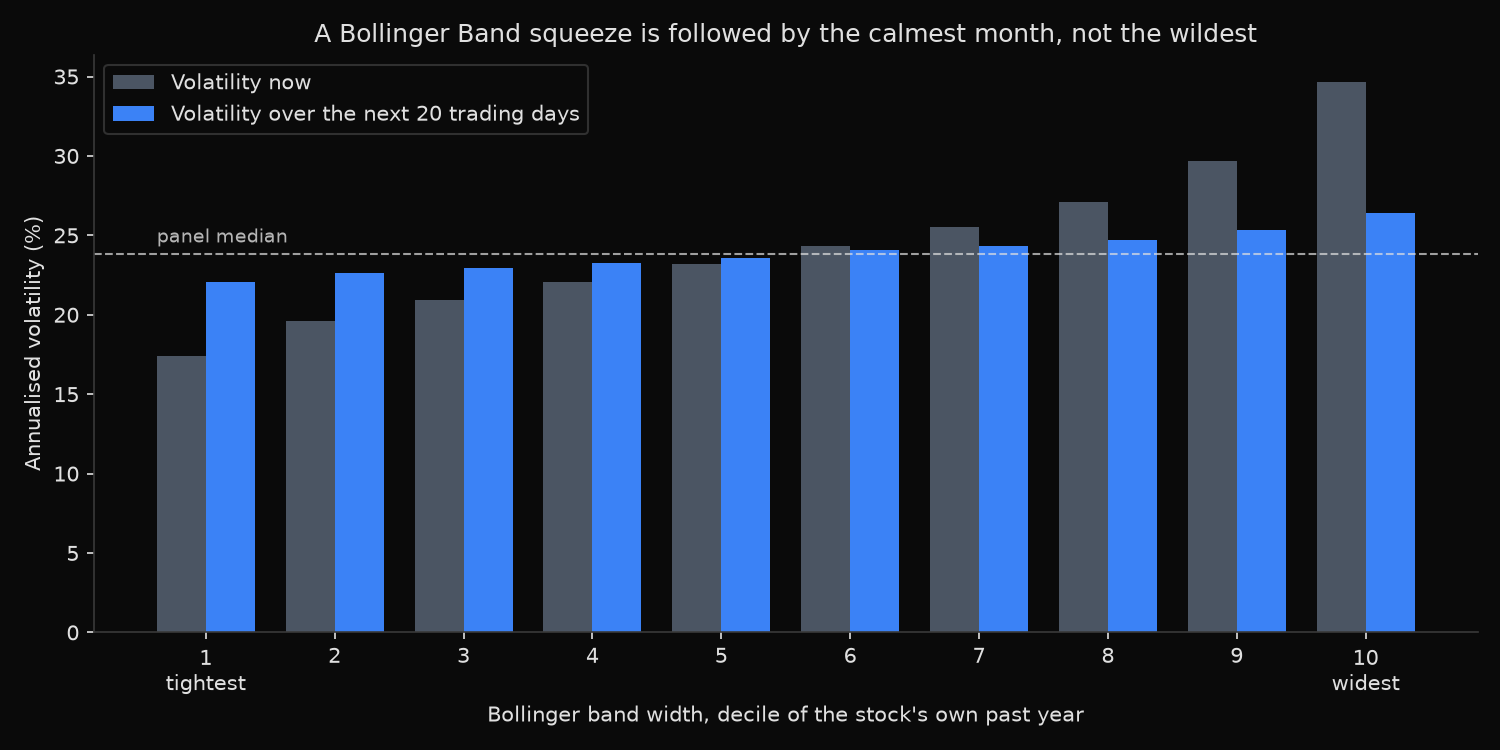
Band width decile          n   Width  Vol now  Vol next   Ratio  |20d move|      Up
 1 tightest          114,017   4.66%    17.4%     22.1%    1.27       4.27%   53.1%
 2                    96,284   6.00%    19.6%     22.6%    1.15       4.42%   54.3%
 3                    95,161   6.96%    20.9%     22.9%    1.10       4.50%   54.6%
 4                    96,010   7.89%    22.1%     23.2%    1.05       4.54%   55.2%
 5                    99,576   8.90%    23.2%     23.6%    1.02       4.55%   55.0%
 6                    96,437  10.03%    24.3%     24.1%    0.99       4.61%   55.5%
 7                    96,157  11.42%    25.5%     24.3%    0.95       4.62%   55.6%
 8                    96,629  13.08%    27.1%     24.7%    0.91       4.70%   55.3%
 9                    99,471  15.69%    29.7%     25.3%    0.85       4.76%   55.8%
10 widest            114,675  21.40%    34.7%     26.4%    0.76       5.06%   56.4%
panel median       1,004,417   9.68%    23.9%     23.9%    1.00       4.60%   55.1%

After a squeeze, volatility rises 27% from its starting point and still lands at 22.1%, the lowest of the ten deciles.
Per company: 444 of 454 expand after a squeeze; 397 of 454 are calmer after a squeeze than after a wide band.

Squeeze-decile ratio of forward to current volatility, by year
2015 1.26  2016 1.33  2017 1.26  2018 1.42  2019 1.21  2020 1.51  2021 1.18  2022 1.15  2023 1.17  2024 1.30

What this tells us

The mean-reversion claim survives. In the tightest decile, realised volatility over the following month runs at 1.27 times the month before: 22.1% against 17.4%. In the widest decile the ratio runs the other way, 0.76, with 26.4% following 34.7%. Both ends converge toward the middle. The pattern holds in all ten calendar years, with the squeeze-decile ratio between 1.15 in 2022 and 1.51 in 2020, and for 444 of the 454 companies that supply observations at both extremes.

The big-move claim fails, in the opposite direction to the folklore. Forward volatility after a squeeze is 22.1%, the lowest figure in the table and below the panel median of 23.9%, while forward volatility after the widest bands is 26.4%, the highest. The ordering runs cleanly from decile 1 to decile 10 without a reversal: the calmer the past month, the calmer the next one tends to be. Median absolute 20-day returns agree, 4.27% after a squeeze against 5.06% after the widest bands.

Both follow from one property: volatility is persistent, so the best simple forecast of next month is this month pulled part of the way toward the long-run average. A squeeze moves a stock part of the way up, not past the average.

Direction carries nothing. Positive forward returns follow a squeeze 53.1% of the time, against 55.1% across the panel and 56.4% after the widest bands. Every decile sits within three points of the base rate.

So what?

Treat a squeeze as a position-sizing input rather than an entry signal. The useful number is the ratio, not the level. After a squeeze, size for volatility roughly 27% above what the last month showed while still expecting a quieter month than average: a stop set at a multiple of trailing volatility will be too tight by about that margin.

For an option seller the same arithmetic is the whole trade. Realised volatility after a squeeze runs a quarter above where it currently sits, so a short straddle priced off trailing realised volatility starts behind on day one. Priced off the panel’s typical forward volatility, 22.1% against 23.9%, it starts ahead.

The breakout trade has the weakest case. A squeeze identifies the calmest state in the sample and is followed by the smallest 20-day moves in the sample, in either direction, with no directional information attached. A breakout system that earns money after squeezes is earning it somewhere else, and finding out where comes before adding size.

Built with xfinlink — free financial data API for Python. pip install -U xfinlink