Do Sectors Diversify When It Matters? Conditional Correlation in Python

August 16, 2026

What’s the question?

Diversification across sectors rests on a simple premise: technology, energy, utilities, and financials do not all move together, so holding several softens the ride. The premise is measured by correlation, the degree to which two return streams move in step. A correlation of 1 means they move identically, 0 means no linear relationship, and a spread of low correlations is what makes a portfolio steadier than its parts.

The premise has a known weakness. Correlation is not a fixed property of two assets. It shifts with market conditions, and the direction of that shift is unkind. When markets are calm, sectors wander on their own stories and correlations are low. When markets fall hard, they tend to fall together, and the diversification that looked solid on a spreadsheet evaporates at the moment it was supposed to help.

This article measures the size of that effect. The question is not whether sector correlations rise in stress, which is well established, but by how much, and whether any sector holds its independence when the others converge.

The approach

The sample is the eleven-year window from January 2016 to December 2025, using SPY for the broad market and the ten sector SPDR funds that partition it: XLK, XLE, XLF, XLV, XLP, XLU, XLI, XLY, XLB, and XLRE. Sector ETFs are cleaner than individual stocks for this purpose, since each already averages away single-company noise and leaves the sector-level co-movement that portfolio construction cares about.

1. Pull daily returns for SPY and the ten sectors, and align them to a common set of trading days.
2. Define the market regime from SPY alone: compute its trailing 20-day annualised volatility, and label the highest third of days "stress" and the rest "calm". Splitting on the market rather than on the sectors themselves keeps the regime definition independent of the correlations being measured.
3. Within each regime, compute the correlation of every pair of sectors and average them, then compute each sector’s average correlation to the other nine.
4. Convert the correlation matrix into an effective number of independent sectors, so the loss of diversification has a single interpretable figure.

The effective number comes from the eigenvalues of the correlation matrix, turned into a diversity score. Ten sectors that moved independently would score 10. Ten sectors that moved as one would score 1. The measure states how many genuinely separate bets the ten funds represent.

Code

import numpy as np
import pandas as pd
import xfinlink as xfl

xfl.set_api_key("YOUR_API_KEY")  # free at https://xfinlink.com/signup

sectors = ["XLK", "XLE", "XLF", "XLV", "XLP", "XLU", "XLI", "XLY", "XLB", "XLRE"]
px = xfl.prices(["SPY"] + sectors, start="2016-01-01", end="2025-12-31",
                fields=["close", "return_daily"], max_rows=200000)

rets = px.pivot_table(index="date", columns="ticker", values="return_daily").dropna()

# regime from the market: top third of SPY 20-day volatility is "stress"
spy_vol = rets["SPY"].rolling(20).std() * np.sqrt(252)
cut = spy_vol.quantile(2 / 3)
regime = pd.Series(np.where(spy_vol >= cut, "stress", "calm"), index=rets.index)
regime = regime[spy_vol.notna()]
sec = rets[sectors].loc[regime.index]

def avg_pairwise_corr(frame):
    c = frame.corr().values
    return c[np.triu_indices_from(c, k=1)].mean()

def effective_n(frame):
    ev = np.linalg.eigvalsh(frame.corr().values)
    ev = ev[ev > 0]
    p = ev / ev.sum()
    return np.exp(-(p * np.log(p)).sum())

for name in ["calm", "stress"]:
    part = sec[regime == name]
    print(name, round(avg_pairwise_corr(part), 3), round(effective_n(part), 2))

Full script with formatting and visualisation: sector-correlations-calm-vs-stress-python.py

Output

SPY + 10 sector SPDRs, daily returns 2016-02-01 to 2025-12-31
2495 trading days with a defined regime (1663 calm, 832 stress)
stress = SPY 20-day annualised volatility in the top third (>= 15.6%)

average pairwise sector correlation, calm   : 0.399
average pairwise sector correlation, stress : 0.731

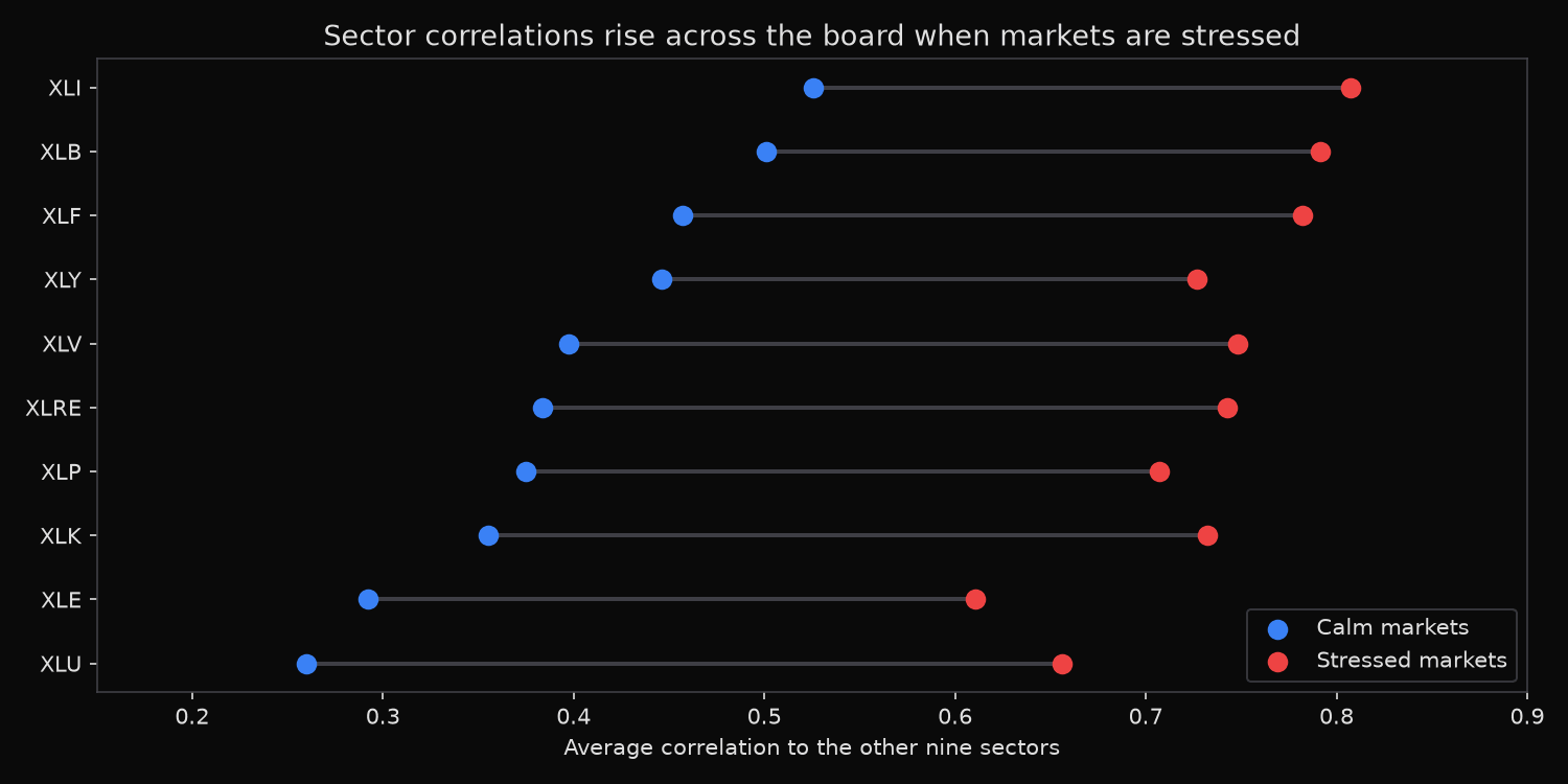
average correlation of each sector to the other nine
sector    calm   stress   rise
XLY     0.446   0.727   +0.281
XLI     0.526   0.807   +0.281
XLB     0.501   0.792   +0.290
XLE     0.292   0.611   +0.318
XLF     0.457   0.782   +0.325
XLP     0.375   0.707   +0.332
XLV     0.397   0.748   +0.351
XLRE    0.384   0.743   +0.359
XLK     0.355   0.732   +0.377
XLU     0.260   0.656   +0.396

effective number of independent sectors, calm   : 5.70 of 10
effective number of independent sectors, stress : 2.71 of 10

What this tells us

Average pairwise correlation nearly doubles, from 0.399 in calm markets to 0.731 in stress. The gap between the two is larger than either number, which is the practical point: the correlation used to size a portfolio in normal conditions understates by a wide margin the correlation that governs it during a drawdown.

The rise is universal. Every one of the ten sectors becomes more correlated with the rest, and the increases fall in a tight band from +0.28 to +0.40. No sector escapes. The two that provide the most diversification in calm markets, utilities at 0.260 and energy at 0.292, are also the two that rise the most, ending at 0.656 and 0.611. Their independence is exactly the property that disappears under stress. Defensive sectors decouple when decoupling is cheap and converge when it is expensive.

The effective number of independent sectors falls from 5.70 to 2.71. A portfolio spread evenly across all ten sectors holds close to six separate bets in calm conditions. During the days that produce the worst losses, the same portfolio behaves like fewer than three. More than half of the apparent diversification is a fair-weather quantity.

The mechanism is systematic risk. In calm periods, returns are driven largely by sector-specific and company-specific news, which is uncorrelated across sectors. In stress, a common factor dominates: a liquidity shock, a policy surprise, or a growth scare moves every risk asset in the same direction at once. Idiosyncratic stories stop mattering when everyone is selling, and the correlation matrix collapses toward one.

So what?

A risk model calibrated on full-history or calm-period correlations will report a portfolio as better diversified than it is when losses arrive. The correlations that matter for tail risk are the stress correlations, not the average ones. Stress-testing a portfolio with a correlation matrix estimated from high-volatility days alone, rather than the full sample, gives a more honest picture of how concentrated the positions become precisely when that concentration bites.

The deeper implication is that diversification across sectors is not a reliable hedge against market-wide declines. It smooths the idiosyncratic bumps of normal markets, which is worth having, but it thins out during systemic events. Protection against those events has to come from genuinely different exposures. Assets whose stress correlation to equities stays low, such as Treasuries or explicit tail hedges, do work that no amount of spreading within the stock market can replicate. The correlation matrix is a moving object, and the version that governs a bad month is the one worth planning around.

Built with xfinlink — free financial data API for Python. pip install -U xfinlink