Does Revenue Concentration Explain Earnings Volatility? Segment Herfindahl Analysis in Python

September 5, 2026

What’s the question?

A company that earns everything from one product line has nowhere to hide when that market turns, while a company with five segments can offset a bad year in one against a good year in another. The claim follows so naturally that analysts assert it in passing, usually to justify a wider discount rate on the focused name.

It is measurable. Companies disclose revenue by reportable operating segment, so concentration can be quantified with a Herfindahl index: square each segment’s share of revenue and add them up. A single-segment filer scores 1.0, four equal segments score 0.25. Set that against how far each company’s earnings actually moved over the past decade, and the assertion either holds or it does not.

The approach

1. Take every company in the S&P 500 on 31 December 2015 or in it now, carried by company identifier so a symbol change does not split one company in two. That gives 661 companies rather than only the ones that stayed in the index.
2. Pull annual filings for all of them with segment detail attached, from fiscal 2015 onward.
3. Measure earnings volatility as the standard deviation of operating income divided by total assets across fiscal 2015 to 2024, requiring at least eight annual observations. Assets are the comparable base here, because a bank, a REIT and a retailer book very different revenue against the same balance sheet.
4. Measure concentration as the Herfindahl index over reportable segment revenue in the most recent annual filing. Single-segment filers score 1.0 by construction, and filings whose segment revenues do not reconcile to the revenue line drop out.
5. Regress volatility on concentration, then add log assets for size, then add sector dummies, reporting the coefficient, t-statistic and R-squared at each step.

Segment structure is read once, from the latest filing, and treated as the shape of the business; reportable segments change rarely, so rebuilding the map year by year would not move the ranking much.

Code

import numpy as np
import pandas as pd
import statsmodels.api as sm
import xfinlink as xfl

xfl.set_api_key("YOUR_API_KEY")  # free at https://xfinlink.com/signup

ids = sorted(set(xfl.index("sp500", as_of="2015-12-31")["entity_id"])
             | set(xfl.index("sp500")["entity_id"]))
fund = pd.concat([xfl.fundamentals(entity_id=ids[i:i + 100], period_type="annual",
                                   start="2015-01-01", include_segments=True,
                                   max_rows=40000)
                  for i in range(0, len(ids), 100)], ignore_index=True)

fund["roa"] = fund["operating_income"] / fund["total_assets"]
hist = (fund[fund["fiscal_year"].between(2015, 2024)].dropna(subset=["roa"])
        .drop_duplicates(["entity_id", "fiscal_year"], keep="last"))
vol = hist.groupby("entity_id").agg(years=("roa", "size"), earn_sd=("roa", "std"),
                                    assets=("total_assets", "mean"),
                                    sector=("gics_sector", "last"))
vol = vol[vol["years"] >= 8]


def hhi(segs):
    if not isinstance(segs, list) or not segs:
        return np.nan
    v = np.array([s["value"] for s in segs], dtype=float)
    v = v[v > 0]
    return np.nan if v.size == 0 else float(((v / v.sum()) ** 2).sum())


latest = fund.sort_values("fiscal_year").groupby("entity_id").tail(1)
latest = latest.assign(
    n_segments=latest["segments_business"].map(
        lambda s: len(s) if isinstance(s, list) else 0),
    hhi=latest["segments_business"].map(hhi),
    coverage=pd.to_numeric(latest["segment_coverage"].map(
        lambda c: c.get("business_pct") if isinstance(c, dict) else None),
        errors="coerce"))
latest.loc[(latest["n_segments"] == 1)
           & latest["coverage"].between(80, 110), "hhi"] = 1.0
keep = latest[latest["coverage"].between(80, 110) & latest["hhi"].notna()]

df = vol.join(keep.set_index("entity_id")[["hhi", "n_segments"]],
              how="inner").dropna(subset=["earn_sd", "hhi", "sector"])
df["log_assets"] = np.log(df["assets"])

for label, X in {
        "concentration only": df[["hhi"]],
        "+ log assets": df[["hhi", "log_assets"]],
        "+ log assets + sector": df[["hhi", "log_assets"]].join(
            pd.get_dummies(df["sector"], drop_first=True, dtype=float))}.items():
    fit = sm.OLS(df["earn_sd"], sm.add_constant(X)).fit()
    print(f"{label:24s} coef={fit.params['hhi']:7.4f} "
          f"t={fit.tvalues['hhi']:6.2f} p={fit.pvalues['hhi']:.3f} "
          f"R2={fit.rsquared:.3f}")

Full script with formatting and visualisation: revenue-concentration-earnings-volatility-python.py

Output

661 companies: S&P 500 membership at 2015-12-31 plus the current roster
6,635 annual filings, 645 companies
549 companies with at least 8 annual observations in 2015-2024
306 companies with reconciling segment revenue in the latest annual filing (30 of them single-segment)
290 companies in the final cross-section, 11 sectors

                           mean   median       sd      min      max
segment Herfindahl        0.559    0.511    0.225    0.152    1.000
earnings volatility       0.042    0.029    0.038    0.003    0.344
mean operating ROA        0.096    0.078    0.084   -0.110    0.724

quartile     n  mean HHI  segments   earn vol  median vol
1           73     0.307       4.2     0.0360      0.0266
2           72     0.453       2.8     0.0422      0.0274
3           72     0.590       2.2     0.0494      0.0390
4           73     0.884       1.7     0.0419      0.0287

specification               HHI coef   t-stat       p      R2
concentration only            0.0066     0.66   0.510   0.002
+ log assets                  0.0064     0.67   0.505   0.078
+ log assets + sector        -0.0006    -0.07   0.947   0.296

Pearson correlation 0.039, Spearman 0.108

sector                        n  mean HHI   earn vol
Communication Services       14     0.622     0.0510
Consumer Discretionary       42     0.617     0.0577
Consumer Staples             21     0.599     0.0332
Energy                       16     0.651     0.1015
Financials                   33     0.549     0.0257
Health Care                  33     0.557     0.0345
Industrials                  49     0.467     0.0345
Information Technology       35     0.512     0.0494
Materials                    17     0.454     0.0498
Real Estate                  11     0.742     0.0215
Utilities                    19     0.592     0.0174

What this tells us

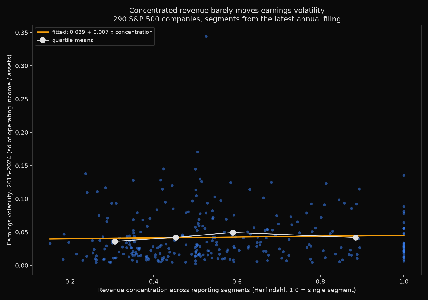
Concentration explains almost nothing: an R-squared of 0.002, a coefficient of 0.0066, a t-statistic of 0.66. Moving a company from four equal segments to a single one, the full width of the measure, raises predicted earnings volatility by about 0.006 against a cross-sectional standard deviation of 0.038. Pearson correlation is 0.039 and rank correlation 0.108.

The quartile means do not line up either. Volatility rises from 0.0360 in the least concentrated quartile to 0.0494 in the third, then falls back to 0.0419 in the most concentrated one. Single-segment filers, the group the argument points at most directly, average less earnings volatility than two-segment companies.

Adding sector settles it. Sector dummies lift R-squared from 0.078 to 0.296 while the concentration coefficient collapses to -0.0006, p-value 0.947. The weak positive association in the raw numbers was concentration sorting by industry.

The sector table holds the cleanest counterexample. Real estate is the most concentrated group at a mean Herfindahl of 0.742, and its earnings volatility of 0.0215 is the second lowest of the eleven sectors; utilities sit at 0.592 concentration and 0.0174 volatility, the lowest of all. Energy sits at almost the same concentration, 0.651, with volatility of 0.1015, roughly six times the utilities figure.

What moves earnings is what a company sells rather than how many things it sells. An oil producer with two segments faces a commodity price that halved twice inside the window; a regulated utility with one segment earns an allowed return on a rate base that moves slowly by design. Diversification inside one firm rarely spans different economic drivers, because segments of the same company sell into related markets and share a cost base.

So what?

Drop segment count from the risk screen. A Herfindahl over reported segments says nothing about how far a company’s earnings will move once industry is known, so ranking candidates by it adds noise rather than caution. The informal version of the same reasoning goes with it: a single-segment filer is not inherently riskier than a multi-segment one.

Sector is the variable that earns its place, accounting for 29.6 percent of the cross-sectional variation in earnings volatility. That is a far better starting point for a cost-of-capital adjustment or a covenant test than the segment table provides. Set the base case from the industry, then adjust for the specific drivers of the business.

Structural proxies that sound like risk, segment count and geographic spread among them, need testing against realised outcomes before they enter a model. This one takes two data pulls and a regression to check, and it failed.

Built with xfinlink — free financial data API for Python. pip install -U xfinlink