Can a Company's Revenue Be Forecast From Its Own History? Out-of-Sample Test in Python

August 29, 2026

What’s the question?

Every valuation model begins with a revenue line, and every revenue line begins with a forecast. Sell-side research builds those forecasts from guidance, channel checks and industry volume models, none of which appears in a company’s own accounts. The accounts set a floor: whatever a mechanical rule achieves from past revenue alone is accuracy no analyst should be credited for.

The rule to beat is the random walk, which forecasts next year’s revenue as this year’s and assumes no growth whatsoever. In many economic series it is close to unbeatable, because whatever sets the level carries forward while whatever sets the change does not.

The alternative is extrapolation: take the growth rate a company just delivered and apply it again. That sits inside most spreadsheet models, and it holds only if growth is persistent, meaning a fast grower this year is likely to grow fast again next year.

The approach

Five rules, each needing nothing but annual revenue history, are scored over ten forecast origins. A forecast made at year t sees revenue through year t and is scored against year t+1.

1. Rebuild the S&P 500 roster at each year end from 2015 to 2024, and use it as the sample for that year’s forecast.
2. Pull annual revenue back to 2008, carried by entity_id rather than by ticker, so a ticker change does not split a series.
3. Anchor each statement to the year it covers using the period end, not the fiscal year label; a year end in January to May belongs to the previous year. Where two annual periods land in one year, keep the one matching the company’s usual year end.
4. Build five forecasts at each origin: no growth; last year’s growth repeated; average growth over four years; last year’s growth shrunk halfway toward the cross-sectional median; and that median applied to every company alike.
5. Score each forecast as absolute percentage error and read the median, since a few mergers move an average by several points on their own.

The panel holds 4,764 forecasts across 630 companies. Because origins overlap in time, each rule’s gain is tested across the ten origin-level medians.

The statements are the restated versions, so a company’s earlier revenue reflects any later reclassification of a division as discontinued. History and the forecast target move together under that convention, which flatters every rule equally and so leaves the ranking between them intact.

Code

import xfinlink as xfl
import pandas as pd
import numpy as np

xfl.set_api_key("YOUR_API_KEY")  # free at https://xfinlink.com/signup

rosters = {y: set(xfl.index("sp500", as_of=f"{y}-12-31")["entity_id"])
           for y in range(2015, 2025)}
universe = sorted(set().union(*rosters.values()))

fu = xfl.fundamentals(entity_id=universe, period_type="annual",
                      start="2008-01-01", end="2026-08-28",
                      fields=["revenue"], max_rows=50000)
fu = fu[fu["revenue"] > 0].copy()

# anchor to the year the period covers, not the fiscal year label
fu["month"] = fu["period_end"].dt.month
fu["y"] = np.where(fu["month"] <= 5, fu["period_end"].dt.year - 1,
                   fu["period_end"].dt.year)
modal = fu.groupby("entity_id")["month"].agg(lambda s: s.mode().iloc[0])
fu["off"] = (fu["month"] - fu["entity_id"].map(modal)).abs()
fu = fu.sort_values(["entity_id", "y", "off"]).drop_duplicates(["entity_id", "y"])

rev = fu.pivot_table(index="entity_id", columns="y", values="revenue")

rows = []
for t in range(2015, 2025):
    for eid in rev.index:
        if eid not in rosters[t]:
            continue
        hist = [rev.at[eid, y] if y in rev.columns else np.nan
                for y in range(t - 4, t + 2)]
        if any(pd.isna(hist)):
            continue
        r = np.asarray(hist, dtype=float)
        g = r[1:5] / r[0:4] - 1           # growth in years t-3 .. t
        rows.append(dict(origin=t, R=r[4], actual=r[5],
                         g_last=g[-1], g_avg=g.mean()))
p = pd.DataFrame(rows)

p["peer"] = p.groupby("origin")["g_last"].transform("median")
models = {"no growth (random walk)": p["R"],
          "last year's growth": p["R"] * (1 + p["g_last"]),
          "4-year average growth": p["R"] * (1 + p["g_avg"]),
          "own growth shrunk halfway": p["R"] * (1 + 0.5 * p["g_last"] + 0.5 * p["peer"]),
          "peer median growth only": p["R"] * (1 + p["peer"])}
ape = pd.DataFrame({k: (v - p["actual"]).abs() / p["actual"] * 100
                    for k, v in models.items()})
print(ape.median().round(2))

Full script with formatting and visualisation: revenue-forecast-own-history-sp500-python.py

Output

point-in-time universe: 680 entities
annual observations 11,017  resolved to one per company-year from 16 overlapping rows
forecasts 4,764  companies 630  origins 2015-2024

out-of-sample absolute percentage error, one year ahead
rule                          median    mean     p75     p90  beats RW
no growth (random walk)         7.31   12.36   13.56   23.71
last year's growth              6.77   19.17   16.26   34.58     50.0%
4-year average growth           6.91   19.03   14.52   30.10     52.0%
own growth shrunk halfway       5.98   14.48   13.05   26.44     56.0%
peer median growth only         6.47   12.17   13.06   24.24     60.4%

gain over the random walk, tested across the ten forecast origins
last year's growth           +0.42pp  wins 7/10  t=+0.84  p=0.421
4-year average growth        +0.47pp  wins 6/10  t=+1.00  p=0.342
own growth shrunk halfway    +1.31pp  wins 8/10  t=+3.00  p=0.015
peer median growth only      +0.81pp  wins 7/10  t=+1.99  p=0.078

next year's growth on this year's growth: slope -0.010  r2=0.000  rank correlation +0.229

growth this year vs growth next year, by decile of this year's growth
  decile  1:  -16.72%  ->   +3.00%
  decile  2:   -3.61%  ->   +2.52%
  decile  3:   -0.54%  ->   +2.90%
  decile  4:   +1.34%  ->   +3.23%
  decile  5:   +3.54%  ->   +4.21%
  decile  6:   +5.79%  ->   +5.28%
  decile  7:   +7.78%  ->   +6.48%
  decile  8:  +10.67%  ->   +6.89%
  decile  9:  +15.90%  ->  +10.12%
  decile 10:  +33.40%  ->  +13.33%

median error by sector, random walk vs the best rule
  Consumer Staples         n= 354  RW   4.49%   shrunk   3.69%
  Utilities                n= 282  RW   6.05%   shrunk   6.56%
  Communication Services   n= 177  RW   6.25%   shrunk   6.01%
  Financials               n= 710  RW   6.77%   shrunk   5.14%
  Industrials              n= 697  RW   6.97%   shrunk   5.50%
  Real Estate              n= 301  RW   7.17%   shrunk   4.48%
  Consumer Discretionary   n= 580  RW   7.28%   shrunk   5.43%
  Health Care              n= 577  RW   7.52%   shrunk   5.42%
  Materials                n= 258  RW   7.85%   shrunk   9.35%
  Information Technology   n= 574  RW   9.50%   shrunk   6.88%
  Energy                   n= 252  RW  19.88%   shrunk  20.23%

median error by revenue size decile at the forecast origin
  decile  1: median revenue $    2.0bn   RW  8.46%   shrunk  5.49%
  decile  2: median revenue $    3.5bn   RW  7.89%   shrunk  5.67%
  decile  3: median revenue $    5.0bn   RW  8.16%   shrunk  6.77%
  decile  4: median revenue $    6.5bn   RW  6.92%   shrunk  6.38%
  decile  5: median revenue $    9.0bn   RW  7.54%   shrunk  6.67%
  decile  6: median revenue $   11.9bn   RW  7.12%   shrunk  6.21%
  decile  7: median revenue $   15.8bn   RW  7.58%   shrunk  6.42%
  decile  8: median revenue $   23.0bn   RW  6.86%   shrunk  6.17%
  decile  9: median revenue $   41.0bn   RW  6.58%   shrunk  5.47%
  decile 10: median revenue $  111.1bn   RW  6.44%   shrunk  4.44%

What this tells us

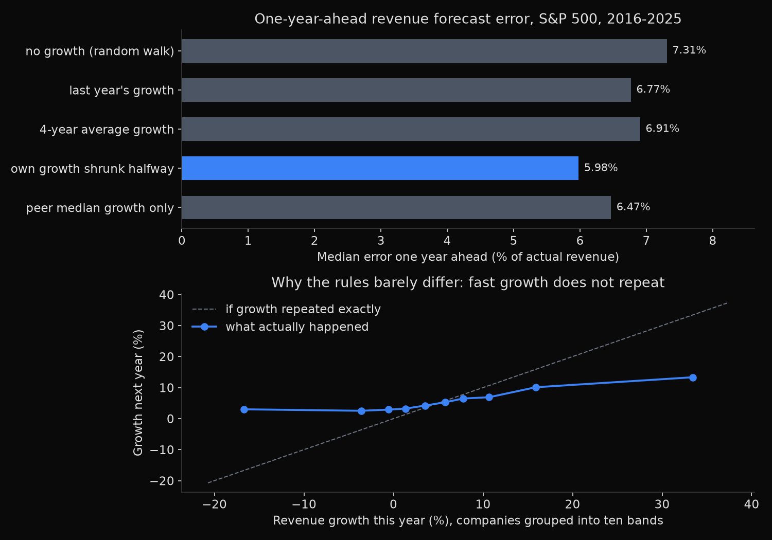
Assuming no growth misses next year’s revenue by 7.31% for the median company. Every rule that tries to beat that lands between 5.98% and 6.91%, so the entire contest is decided inside 1.33 percentage points.

Extrapolating last year’s growth is the rule most models use and the one the data supports least. Its median error improves to 6.77%, while its mean rises from 12.36% to 19.17% and its 90th percentile from 23.71% to 34.58%. Across the ten origins its average gain of 0.42 percentage points carries a t-statistic of 0.84.

The second panel explains why. Regressing next year’s growth on this year’s produces a slope of −0.010 and an r-squared of 0.000. Companies in the fastest-growing decile grew 33.40% and then 13.33%; the slowest decile shrank 16.72% and then grew 3.00%. A rank correlation of +0.229 says that ordering carries a little information; the size of a growth rate carries almost none.

Shrinkage repairs most of the damage. Halving the company’s own growth rate and replacing the other half with the cross-sectional median cuts the median error to 5.98% and wins in 8 of 10 origins, at a p-value of 0.015. The last row matters most: the peer median applied to every company alike recovers 0.81 of that 1.31 point gain on its own, so three fifths of the apparent improvement is a constant every company shares rather than anything specific to the company being forecast.

Forecastability is uneven. Consumer Staples sits at 4.49% under the random walk against 19.88% for Energy, whose revenue is a volume times a commodity price the company does not set. Shrinkage helps in eight sectors and hurts in three, and the three it hurts are Energy, Materials and Utilities, all of them commodity-linked. The largest revenue decile records 6.44% against 8.46% for the smallest.

So what?

The number to carry away is 6%. A revenue forecast for a large-cap company that lands within 6% of the outcome has matched an arithmetic rule that reads two revenue figures off an income statement and blends them with a number every company in the sample shares. Judging a research process against zero error flatters it; 5.98% is the honest bar, and a machine learning model must clear the shrunk rule, not the random walk.

For forecasts built at scale, use the shrunk form and never carry a growth rate forward at full weight; the cost of full extrapolation appears in the tail, which is where a portfolio gets hurt.

Sizing the uncertainty matters as much as the point estimate. The 90th percentile error at one year is 26.44% under the best rule, so a discounted cash flow model that varies revenue by five percent either side tests a band reality escapes one year in four. Widen it, more so for Energy and Materials.

Built with xfinlink — free financial data API for Python. pip install -U xfinlink