Does Post-Earnings Announcement Drift Survive Real Filing Dates? PEAD Event Study in Python

July 26, 2026

What's the question?

Post-earnings announcement drift (PEAD) is the finding that companies reporting unexpectedly strong results keep outperforming for weeks afterwards, while those that disappoint keep lagging. Ball and Brown documented it in 1968 and it has been re-tested ever since.

Testing it requires choosing a date, and this is where most backtests go wrong. They use the fiscal period end, because every dataset carries that field. A company whose quarter closes on 31 March does not tell anybody what it earned on 31 March; the numbers become public when the filing lands on EDGAR, typically a month later. A 60-day window starting at the period end therefore contains the announcement itself, which is the largest single move of the whole episode. Returns booked inside that window were unavailable to anybody trading the results, because the results were not public yet.

So: how much of measured drift is drift, and how much is announcement reaction smuggled in by a careless clock?

The approach

No analyst estimates enter this test. The expectation has to come from a company’s own record, which gives standardised unexpected earnings (SUE) built on a seasonal random walk: the expected figure for a quarter is the same quarter one year earlier. That is a time-series proxy for surprise, not an estimate-based one.

1. 40 large caps across technology, healthcare, energy, financials, staples and industrials, using quarterly net income from 2013 onward.
2. Net income rather than per-share earnings, since a share count resetting at a stock split makes per-share figures non-comparable year over year.
3. Unexpected earnings is net income minus the same quarter a year prior, standardised by the dispersion of that company’s own past year-over-year changes, lagged one quarter so no event contaminates its own scale. At least 8 prior changes required.
4. Keep quarters whose filing date falls 1 to 120 days after the period end, the statutory reporting window. filing_date records the filing a figure came from, which for a restated quarter can be a later comparative filing.
5. Sort events into SUE quintiles, then measure cumulative abnormal return as the daily return minus SPY summed across 60 trading days from the day after the event.
6. Run it twice: clock at filing_date, then at period_end.

WMT retains too few quarters inside that window to standardise and drops, leaving 39 names and 934 events from January 2018 to April 2026, dominated by interim quarters.

Code

import numpy as np
import pandas as pd
from scipy.stats import ttest_ind
import xfinlink as xfl

xfl.set_api_key("YOUR_API_KEY")  # free at https://xfinlink.com/signup

TICKERS = ["AAPL", "MSFT", "GOOGL", "AMZN", "META", "NVDA", "JPM", "JNJ", "V",
           "PG", "XOM", "HD", "CVX", "MRK", "ABBV", "PEP", "KO", "WMT", "COST",
           "MCD", "CSCO", "ADBE", "CRM", "TXN", "QCOM", "AMD", "INTC", "NKE",
           "UNH", "LIN", "HON", "CAT", "LMT", "BA", "GE", "UPS", "MMM", "T",
           "VZ", "DIS"]
HORIZON, MIN_HISTORY, MAX_LAG = 60, 8, 120

fun = xfl.fundamentals(TICKERS, period_type="quarterly", start="2013-01-01",
                       fields=["net_income", "filing_date", "period_end"])
fun = fun.drop_duplicates(subset=["ticker", "fiscal_year", "fiscal_period"])
fun = fun.dropna(subset=["net_income", "filing_date", "period_end"])
fun["lag"] = (fun["filing_date"] - fun["period_end"]).dt.days
fun = fun[(fun["lag"] > 0) & (fun["lag"] <= MAX_LAG)]

# seasonal random walk: expectation is the same fiscal quarter one year ago
prev = fun[["ticker", "fiscal_year", "fiscal_period", "net_income"]].copy()
prev["fiscal_year"] += 1
prev = prev.rename(columns={"net_income": "net_income_yoy"})
ev = fun.merge(prev, on=["ticker", "fiscal_year", "fiscal_period"], how="inner")
ev["ue"] = ev["net_income"] - ev["net_income_yoy"]
ev = ev.sort_values(["ticker", "period_end"])

# shift(1) keeps the current event out of its own scaling factor
ev["scale"] = ev.groupby("ticker")["ue"].transform(
    lambda s: s.shift(1).expanding(MIN_HISTORY).std())
ev = ev.dropna(subset=["scale"])
ev = ev[ev["scale"] > 0]
ev["sue"] = ev["ue"] / ev["scale"]

universe = sorted(ev["ticker"].unique())
series = {t: xfl.prices(t, start="2017-06-01", fields=["return_daily"])
          .set_index("date")["return_daily"] for t in universe + ["SPY"]}

# SPY defines the trading calendar; abnormal return is the excess over it
cal = np.array(sorted(series["SPY"].index.unique()))
spy = series["SPY"].reindex(cal)
excess = {t: (series[t].reindex(cal) - spy).to_numpy() for t in universe}

def car(ticker, event_date):
    i = int(np.searchsorted(cal, np.datetime64(event_date), side="right"))
    if i + HORIZON > len(cal):
        return None
    return np.cumsum(excess[ticker][i:i + HORIZON])

rows = []
for r in ev[ev["filing_date"] >= "2018-01-01"].itertuples():
    a, b = car(r.ticker, r.filing_date), car(r.ticker, r.period_end)
    if a is None or b is None:
        continue
    rows.append({"sue": r.sue, "car_filing": a[-1], "car_period": b[-1]})

res = pd.DataFrame(rows)
res["bucket"] = pd.qcut(res["sue"], 5, labels=["Q1 low", "Q2", "Q3", "Q4",
                                               "Q5 high"])
print(res.groupby("bucket", observed=True)[["car_filing", "car_period"]]
      .mean().mul(100).round(2).to_string())

for col in ("car_filing", "car_period"):
    top = res.loc[res["bucket"] == "Q5 high", col]
    bot = res.loc[res["bucket"] == "Q1 low", col]
    t, p = ttest_ind(top, bot, equal_var=False)
    print(f"{col}: spread {(top.mean() - bot.mean()) * 100:.2f}%  "
          f"t={t:.2f}  p={p:.3f}")

Full script with formatting and visualisation: post-earnings-announcement-drift-filing-date-python.py

Output

Post-earnings announcement drift | seasonal random walk SUE | 60 trading days
universe 39 large caps | events 934 | 2018-01-05 to 2026-04-27
filing lag after period end: median 30d  p5 22d  p95 38d
quarters kept by the 1-120d statutory window screen: 1723 of 2120

SUE bucket  events  mean SUE  CAR from filing  CAR from period end  pre-filing leg
Q1 low         187     -2.22           -0.02%               -1.32%          -1.74%
Q2             187     -0.20            0.53%               -1.83%          -1.46%
Q3             186      0.28           -0.69%               -0.55%          -0.37%
Q4             187      0.91            1.00%                1.86%           1.25%
Q5 high        187      3.05            1.43%                1.65%           1.23%

top-minus-bottom spread from filing date:    1.45%
top-minus-bottom spread from period end:     2.97%
inflation from timing off period end:        1.53%  (2.05x)
top-minus-bottom spread, pre-filing leg:     2.97%  (the announcement reaction the period-end clock swallows)

Welch test on the top-minus-bottom spread
  from filing date:  t =  1.11   p = 0.266
  from period end:   t =  2.23   p = 0.026

events by fiscal quarter: Q1 310  Q2 308  Q3 303  Q4 13
CAR range across all events: -55.8% to 53.4%
NaN check | sue 0  car_filing 0  car_period 0

What this tells us

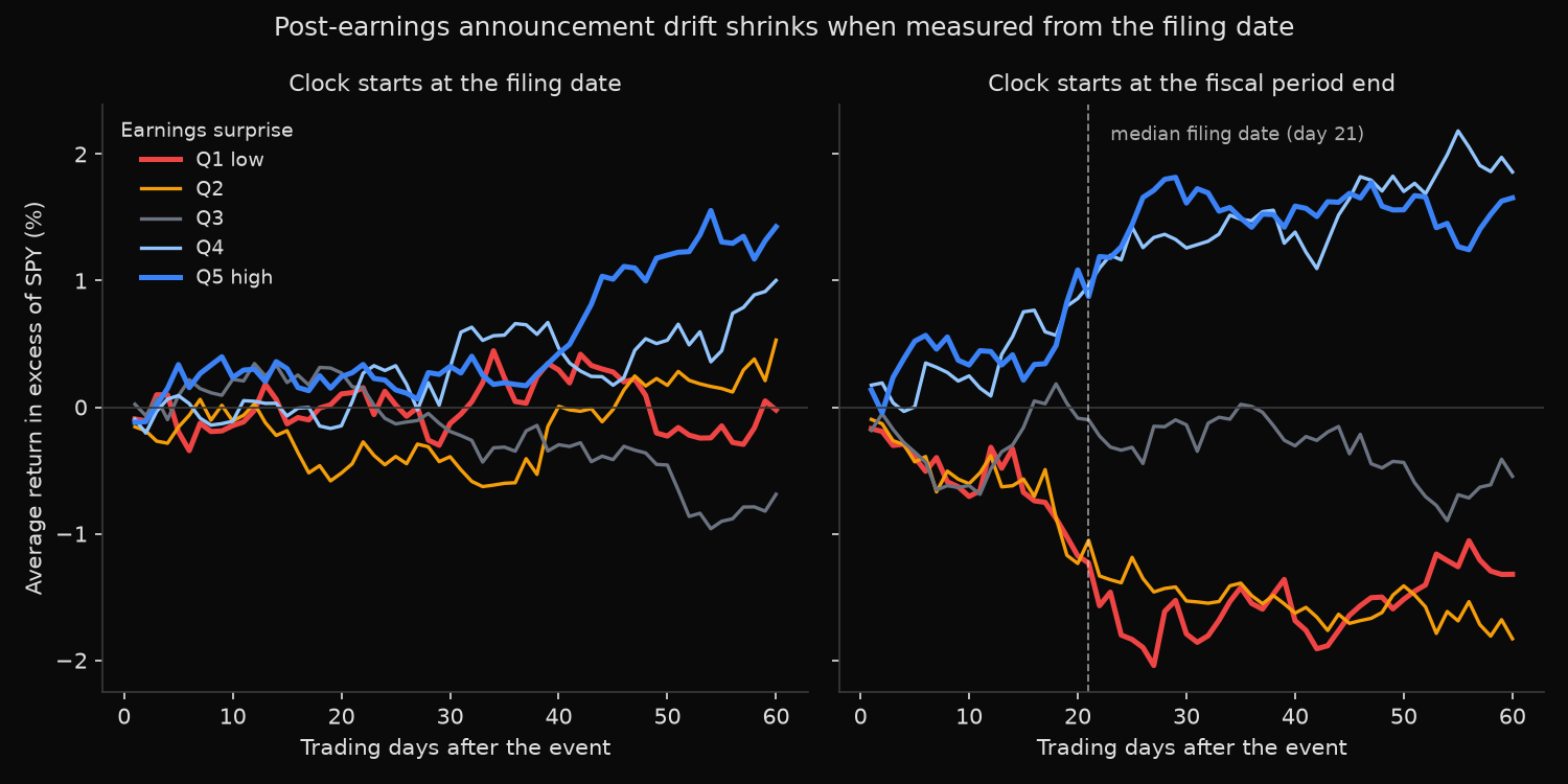
In the right panel the quintiles separate cleanly, and the separation begins around day 21, which is the median trading-day offset between period end and filing date. The ordering does not emerge because the market slowly digested stale news. It emerges the moment the news enters the measurement window.

The top-minus-bottom spread is 2.97% from the period end against 1.45% from the filing date, so the naive clock roughly doubles the answer. Significance moves further than magnitude does: from the period end the spread carries t = 2.23 and p = 0.026, clearing the conventional threshold, while from the filing date it drops to t = 1.11 and p = 0.266. Shifting the start date by three weeks converts a publishable result into noise.

The pre-filing column isolates the mechanism, measuring excess return between period end and filing date only. That is the stretch the naive clock banks before an honest clock starts, and its top-minus-bottom spread of 2.97% matches the full period-end spread almost exactly. Everything the naive version appears to earn arrives before the filing.

What remains is small and imperfectly ordered: Q5 high delivers +1.43% against -0.02% for Q1 low, while Q2 at +0.53% sits above Q3 at -0.69%. Weak and non-monotonic is the expected result here. PEAD was always strongest among small, thinly followed stocks, and decades of publication have competed most of it out of mega caps like these.

So what?

Key any fundamental event study off the filing date. A backtest built on period ends cannot separate drift from reaction even in principle, which makes its headline number untestable rather than merely optimistic.

Treat the 2.05x gap as calibration for what other silent look-ahead is worth. A three-week timing error, introduced by nothing more sinister than using the field that happened to be present, doubled a spread and flipped its p-value.

The honest number does not support trading PEAD in this universe. A 1.45% spread over three months, before costs, with p = 0.266, is not an edge. Two directions remain worth testing: smaller and less covered names where the anomaly was originally strongest, and horizons much shorter than 60 days, where any genuine drift should concentrate.

Built with xfinlink — free financial data API for Python. pip install xfinlink