
Survivorship bias inflates all three weighting rules in an S&P 500 portfolio optimization backtest, and each optimizer moves it by less than 1.3 points a year from equal weight’s. Building each January’s portfolio from the end-2024 constituents instead of the roster of the time adds 6.44 percentage points a year to maximum Sharpe over 2000-2024, 5.20 to equal weight and 3.92 to minimum variance. Each bias is significant (t from 4.25 to 7.55); neither optimizer’s bias differs significantly from equal weight’s (t = 1.65 and -1.27).
Does an optimizer amplify survivorship bias or dampen it?
Survivorship bias is the error of testing on a universe chosen with knowledge of the future. A list of today’s index members omits companies that later failed or were taken over, and it holds others years before they joined. A common optimization exercise takes today’s tickers, downloads their history and runs the recipe that libraries such as PyPortfolioOpt make short: a Ledoit-Wolf covariance matrix, then max_sharpe() or min_volatility().
Two forces pull against each other. A capped optimizer holds roughly 45 to 60 names rather than 480, so it can sidestep many later failures; yet it picks by past behaviour, and on a survivor list the past winners include companies whose climb is already known to have continued.
Twenty-five January portfolios on two universes
- Rebalance on the first trading day of each January, 2000 to 2024. The point-in-time universe is the S&P 500 on that date, as in the historical S&P 500 constituents lookup, drawn with
as_ofper the index membership reference. The survivor universe is the end-2024 list at every date. A third, members of the time still on the end-2024 list, splits the bias in two. - In both universes a name needs 60 complete monthly total returns ending the previous December and a priced January: 459 to 491 names point-in-time, 288 to 481 on the survivor list.
- Rules: equal weight, long-only minimum variance, and long-only maximum Sharpe on trailing 60-month means. The optimizers use a Ledoit-Wolf covariance matrix (Journal of Multivariate Analysis, 2004), shrunk toward a scaled identity, and cap each name at 5%.
- Buy and hold for twelve months on monthly total returns by
entity_id. A holding that stops trading gets its recorded delisting return, then its proceeds follow SPY to the year end. Members removed from the index but still trading stay held. A month without a recorded close carries a holding at its last close. - Report annualised return, volatility and Sharpe ratio (zero risk-free rate) over 300 months. The bias is survivor minus point-in-time, with a paired t-statistic on the 25 yearly differences.
A comparison of cap-weighted and equal-weight backtests treats the same problem under monthly rebalancing, and an out-of-sample test of mean-variance optimisation sets these optimizers against equal weight on the rosters of the time.
Code
import numpy as np
import pandas as pd
import xfinlink as xfl

xfl.set_api_key("YOUR_API_KEY")  # free at https://xfinlink.com/signup
xfl.set_timeout(300)

HIST, CAP = 60, 0.05            # months of history a name needs; per-name weight cap
YEARS = range(2000, 2025)

# ---- data ---------------------------------------------------------------------------------
spy = xfl.prices("SPY", start="1994-12-01", end="2024-12-31", interval="1mo", fields=["return_daily"])
jan = spy.loc[(spy["date"].dt.month == 1) & spy["date"].dt.year.between(2000, 2024), "date"]
roster = {d.year: set(xfl.index("sp500", as_of=d.date().isoformat())["entity_id"].dropna().astype(int))
          for d in jan}                                                   # members on each rebalance date
end24 = set(xfl.index("sp500", as_of="2024-12-31")["entity_id"].dropna().astype(int))

ids = sorted(set().union(*roster.values(), end24))
px = pd.concat([xfl.prices(entity_id=ids[i:i + 150], start="1995-01-01", end="2024-12-31", interval="1mo",
                           fields=["return_daily"], max_rows=400_000) for i in range(0, len(ids), 150)])
px["m"] = px["date"].dt.to_period("M")
px = px.drop_duplicates(["entity_id", "m"])
R = px.pivot(index="m", columns="entity_id", values="return_daily").sort_index()
last = px.dropna(subset=["return_daily"]).groupby("entity_id")["m"].max()   # last priced month
spy_r = spy.assign(m=spy["date"].dt.to_period("M")).set_index("m")["return_daily"]

# Exit records (meta.delisting) for series that end before December 2024, one call per exit year
ended = last[(last >= pd.Period("2000-01", "M")) & (last < pd.Period("2024-12", "M"))]
delist = {}
for y, g in ended.groupby(ended.dt.year):
    g = g.index.tolist()
    for i in range(0, len(g), 150):
        d = xfl.prices(entity_id=g[i:i + 150], start=f"{y}-01-01", end="2024-12-31", interval="1mo",
                       fields=["return_daily"])
        delist.update({int(k): v.get("delisting_return") for k, v in (d.attrs["meta"].get("delisting") or {}).items()})


# ---- estimation and optimisation ----------------------------------------------------------
def ledoit_wolf(X):
    """Ledoit-Wolf (2004) shrinkage of the sample covariance toward a scaled identity."""
    X = X - X.mean(0)
    T, N = X.shape
    S = X.T @ X / T
    m = np.trace(S) / N
    d2 = ((S - m * np.eye(N)) ** 2).sum() / N
    b2 = min(((np.einsum("ti,ti->t", X, X) ** 2).sum() - T * (S ** 2).sum()) / (T * T * N), d2)
    return b2 / d2 * m * np.eye(N) + (1 - b2 / d2) * S


def project(v, cap):
    """Euclidean projection onto {0 <= w <= cap, sum(w) = 1}, by bisection on the shift."""
    lo, hi = v.min() - 1, v.max()
    for _ in range(50):
        t = (lo + hi) / 2
        lo, hi = (t, hi) if np.clip(v - t, 0, cap).sum() > 1 else (lo, t)
    return np.clip(v - (lo + hi) / 2, 0, cap)


def frontier(S, mu, lam, cap, iters=3000):
    """Accelerated projected gradient for max mu'w - lam/2 w'Sw on the capped simplex."""
    step = 1 / (lam * np.linalg.eigvalsh(S)[-1])
    w = z = np.ones(len(S)) / len(S)
    t = 1.0
    for _ in range(iters):
        w1 = project(z - step * (lam * S @ z - mu), cap)
        t1 = (1 + (1 + 4 * t * t) ** 0.5) / 2
        z, w, t = w1 + (t - 1) / t1 * (w1 - w), w1, t1
    return w


def min_var(S, cap):
    return frontier(S, np.zeros(len(S)), 1.0, cap)


def max_sharpe(mu, S, cap):
    """Highest mu'w / sqrt(w'Sw) on the capped-simplex frontier: grid, then golden section on log(lam)."""
    f = lambda x: (lambda w: (mu @ w) / np.sqrt(w @ S @ w))(frontier(S, mu, np.exp(x), cap, 1500))
    grid = np.linspace(-2, 9, 23)
    i = int(np.argmax([f(x) for x in grid]))
    assert 0 < i < len(grid) - 1, "optimum at the edge of the search grid"
    a, b, g = grid[i - 1], grid[i + 1], (5 ** 0.5 - 1) / 2
    for _ in range(14):
        c, d = b - g * (b - a), a + g * (b - a)
        a, b = (a, d) if f(c) > f(d) else (c, b)
    return frontier(S, mu, np.exp((a + b) / 2), cap)


def hold(ids, w, y):
    """Buy and hold for 12 months. A holding that stops trading gets its delisting return,
    then its proceeds follow SPY; a month with no recorded close carries it at its last close."""
    months = pd.period_range(f"{y}-01", f"{y}-12", freq="M")
    H = R.reindex(index=months, columns=ids)
    V, info = [], []
    for e in ids:
        k = (last[e] - months[0]).n if last[e] < months[-1] else 11       # last priced month
        v = np.cumprod(1 + np.nan_to_num(H[e].to_numpy()[:k + 1]))
        dr = delist.get(e) if k < 11 else None
        if k < 11:
            v[-1] *= 1 + (dr if dr is not None and not np.isnan(dr) else 0.0)
            v = np.r_[v, v[-1] * np.cumprod(1 + spy_r.reindex(months[k + 1:]).to_numpy())]
        V.append(v)
        info.append((e, k < 11, dr, v[-1] - 1))
    P = np.r_[1.0, w @ np.array(V)]
    return P[1:] / P[:-1] - 1, pd.DataFrame(info, columns=["id", "exit", "dr", "yr"]).assign(w=w)


UNIV = {"Point-in-time": lambda y: roster[y], "End-2024 list": lambda y: end24,
        "Members then, in end-2024 list": lambda y: roster[y] & end24}
RULES = ["Equal weight", "Minimum variance", "Maximum Sharpe"]


def run(task):
    y, u = task
    est = R.loc[pd.Period(f"{y - 1}-12", "M") - HIST + 1: pd.Period(f"{y - 1}-12", "M")]
    ids = sorted(e for e in UNIV[u](y) if e in est.columns and est[e].notna().all()
                 and last[e] >= pd.Period(f"{y}-01", "M"))                # full history, trades in January
    X = est[ids].to_numpy()
    S, mu = ledoit_wolf(X), X.mean(0)
    book = {"Equal weight": np.ones(len(ids)) / len(ids), "Minimum variance": min_var(S, CAP),
            "Maximum Sharpe": max_sharpe(mu, S, CAP)}
    return [((u, rule, y), len(ids), *hold(ids, w, y)) for rule, w in book.items()]


tasks = [(y, u) for y in YEARS for u in UNIV]
res = [o for t in tasks for o in run(t)]
monthly = {k: r for k, _, r, _ in res}
Hd = pd.concat([h.assign(u=k[0], rule=k[1], year=k[2]) for k, _, _, h in res], ignore_index=True)
Hd["left"] = ~Hd["id"].isin(end24)                                    # not in the end-2024 list
Hd["notyet"] = [e not in roster[y] for e, y in zip(Hd["id"], Hd["year"])]

def stats(u, rule):
    r = np.concatenate([monthly[(u, rule, y)] for y in YEARS])
    yr = np.array([np.prod(1 + monthly[(u, rule, y)]) - 1 for y in YEARS])
    return np.prod(1 + r) ** (12 / len(r)) - 1, r.std(ddof=1) * 12 ** 0.5, r.mean() / r.std(ddof=1) * 12 ** 0.5, yr

tstat = lambda d: d.mean() / d.std(ddof=1) * len(d) ** 0.5
S = {(u, rule): stats(u, rule) for u in UNIV for rule in RULES}
gap = {rule: S[("End-2024 list", rule)][3] - S[("Point-in-time", rule)][3] for rule in RULES}
bias = {rule: S[("End-2024 list", rule)][0] - S[("Point-in-time", rule)][0] for rule in RULES}
for rule in RULES:
    print(rule, [f"{v:.2%}" for v in S[("Point-in-time", rule)][:2] + S[("End-2024 list", rule)][:2]],
          f"bias {bias[rule]:+.2%}", f"t={tstat(gap[rule]):.2f}")
Full script with formatting and visualisation: portfolio-optimization-survivorship-bias-python.py
Output
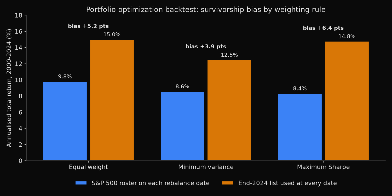
Rebalances: first trading day of January, 2000-2024; 60 monthly returns required; cap 5% a name; Sharpe at a zero risk-free rate
Names per rebalance: point-in-time 459-491, end-2024 list 288-481

                     point-in-time rosters           end-2024 list           bias, points a year
                     return     vol Sharpe   return     vol Sharpe    annual  mean gap     t  ahead
Equal weight          9.83%  16.71%  0.647   15.03%  15.67%  0.977     +5.20     +4.96  7.55  24/25
Minimum variance      8.59%  12.21%  0.739   12.51%  11.91%  1.054     +3.92     +4.01  4.25  20/25
Maximum Sharpe        8.35%  13.77%  0.654   14.80%  14.22%  1.047     +6.44     +6.64  6.28  24/25
Bias against equal weight's, year by year: minimum variance -0.94 (t = -1.27), maximum Sharpe +1.68 (t = 1.65)

Bias split, points a year: dropping members later removed / adding companies not yet members
  Equal weight       +2.25 / +2.95
  Minimum variance   +1.15 / +2.77
  Maximum Sharpe     +1.89 / +4.55

Weight on each slice (mean over 25 rebalances) and its weighted mean 12-month return
  Equal weight      point-in-time, later removed  35.5%   +7.2%   end-2024 list, not yet members  23.8%  +25.4%
  Minimum variance  point-in-time, later removed  25.3%   +6.5%   end-2024 list, not yet members  23.4%  +23.5%
  Maximum Sharpe    point-in-time, later removed  27.9%   +3.6%   end-2024 list, not yet members  31.8%  +26.9%

Point-in-time holdings that stopped trading inside their year: 271, 269 with a recorded delisting return
Where each optimizer put its weight
Minimum variance carries the smallest bias. It gave 25.3% of its point-in-time weight to members gone from the index by the end of 2024, against 35.5% for equal weight, and dropping those names moves it by 1.15 points rather than 2.25.
Maximum Sharpe carries the largest, mostly from the other side. On the end-2024 list it put 31.8% of its weight in companies not yet in the index, against 23.8% for equal weight, and those holdings returned 26.9% over the next twelve months on average. The optimizer chose them for their trailing returns, and a survivor list holds only the climbers that kept climbing: adding them is worth 4.55 points, against 2.95 under equal weight. On the real rosters, its later-removed holdings averaged 3.6% a year, half equal weight’s 7.2%.
The ranking against equal weight is not secure. Maximum Sharpe’s excess over equal weight falls to 0.76 points (t = 0.47) with a 36-month estimation window and is 1.41 (t = 1.24) with a 10% cap; the order holds in both.
Comparing weighting rules without a survivor list
On the rosters of the time the three rules span 8.35% to 9.83% a year. The survivor list adds 3.92 to 6.44 points to each, more than that whole range, and it changes the verdict on maximum Sharpe: on the end-2024 list it leads equal weight by 0.070 in Sharpe ratio, on the real rosters by 0.007. Minimum variance led equal weight in Sharpe ratio on both.
Rebuild the universe from the roster on each rebalance date before comparing optimizers, follow holdings by entity_id, and apply the delisting return when one stops trading. An optimizer run on today’s tickers mostly measures the ticker list. An analysis of stocks removed from the S&P 500 covers the companies such a list leaves out.
Built with xfinlink — free financial data API for Python.