
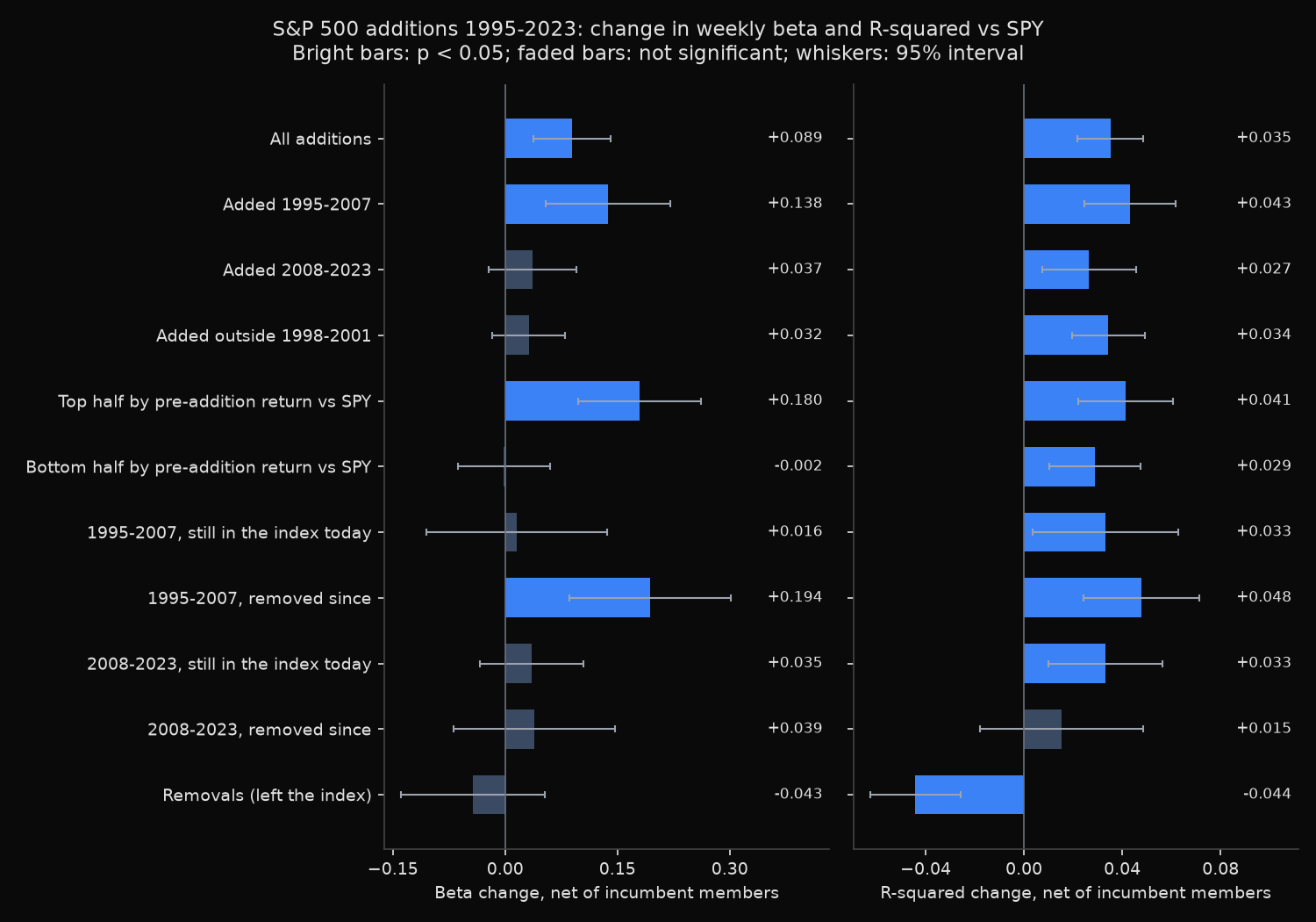
A stock that joins the S&P 500 moves more closely with the index afterwards, but its beta rises by less than the headline average suggests. Across 612 additions from 1995 to 2023, the share of weekly return variance explained by SPY (R-squared) rose 0.035 more than for incumbent members over the same weeks (t 5.17), and 265 stocks that left show the mirror image, −0.044 (t −4.71). Beta rose 0.089 net of incumbents (t 3.37), but outside the additions of 1998-2001 the rise is 0.032 and not significant.
Does a stock start moving with the S&P 500 once it joins?
Beta is how far a stock moves for each 1% market move; R-squared is the fraction of its variance the market explains. If joining changes them, a pre-addition estimate used for hedging is stale on day one.
Vijh (Review of Financial Studies, 1994) found that weekly betas of stocks added in 1985-1989 rose by 0.130 on average. Barberis, Shleifer and Wurgler (“Comovement”, Journal of Financial Economics, 2005) report that an added stock’s beta and R-squared with the index increase, and the converse on deletion. Kasch and Sarkar (New York Fed Staff Report 484) counter that added firms arrive with strong earnings and price momentum, and that net of this, inclusion has no permanent effect on comovement. The test needs every addition, including those later removed or acquired.
Measuring 612 additions against incumbents over the same weeks
- Pull every dated S&P 500 addition and removal with
xfl.index_events(index events reference), keeping 1995-2023 events whose post-event window ends in 2024. - Use weekly total returns for each event stock and SPY, which damps noise from thinly traded stocks.
- Estimate beta and R-squared against SPY over weeks −56 to −5 and +5 to +56; the four skipped weeks on each side hold the announcement and the rebalancing trades. Additions without 52 priced weeks on each side drop from the sample, which excludes fresh spin-offs and IPOs.
- Each event year, draw 60 stocks that were members for the whole window (
xfl.index("sp500", as_of=...), the rosters behind the historical S&P 500 constituents lookup) and subtract their average change over identical weeks. A second control compares incumbents with the same starting beta, since measured betas drift back toward 1. - Run t-tests and Wilcoxon signed-rank tests, also on the 29 cohort-year averages, since windows overlap. Split by period, by pre-addition return against SPY, and by membership today.
Removals are measured the same way if the stock traded 56 weeks after leaving.
Code
import numpy as np
import pandas as pd
import xfinlink as xfl
from scipy import stats

xfl.set_api_key("YOUR_API_KEY")  # free at https://xfinlink.com/signup

LAST_WEEK = pd.Timestamp("2024-12-23")     # every post window ends inside 2024
SKIP, N = 4, 52                            # skip 4 weeks either side of the event, then 52 weeks
rng = np.random.default_rng(0)


def weekly(px):
    """Weekly total returns keyed on the Monday of each week, one column per security."""
    px = px.dropna(subset=["return_daily"]).copy()
    px["week"] = px["date"] - pd.to_timedelta(px["date"].dt.day_of_week, unit="D")
    return px.groupby(["entity_id", "week"])["return_daily"].apply(lambda r: np.prod(1 + r) - 1).unstack(0)


# 1. Every S&P 500 addition and removal since 1990 (offset paging, 1,000 rows a call; the
# "returned 1000 of 1675 rows" warning on the first call is expected, the second call fetches the rest)
pages = [xfl.index_events("sp500", start="1990-01-01", end="2024-12-31", limit=1000, offset=o) for o in (0, 1000)]
ev = pd.concat(pages, ignore_index=True)
ev["d"] = pd.to_datetime(ev["effective_date"])
ev["year"] = ev["d"].dt.year


def member(e, t):
    """Was security e in the index on date t, read off its own dated events."""
    x = ev[ev["entity_id"] == e].sort_values("d")
    before, after = x[x["d"] <= t], x[x["d"] > t]
    if len(before):
        return before["event_type"].iloc[-1] == "added"
    return len(after) > 0 and after["event_type"].iloc[0] == "removed"


# 2. Weekly returns: SPY, the event stocks and 60 incumbents per cohort year
spy = weekly(xfl.prices("SPY", start="1993-01-01", end="2024-12-31", interval="1w", fields=["return_daily"])).iloc[:, 0]
stock_r, ctrl_r = {}, {}
for y in range(1995, 2024):
    start, end = f"{y - 2}-10-01", min(f"{y + 2}-03-31", "2024-12-31")
    ids = sorted(set(ev.loc[ev["year"] == y, "entity_id"].astype(int)))
    stock_r[y] = weekly(xfl.prices(entity_id=ids, start=start, end=end, interval="1w",
                                   fields=["return_daily"], max_rows=200_000))
    ro = xfl.index("sp500", as_of=start)                          # roster when the cohort's window opens
    inc = ro[ro["removed_date"].isna() | (ro["removed_date"] >= end)]  # members for the whole window
    pick = sorted(rng.choice(inc["entity_id"].dropna().astype(int).unique(), 60, replace=False).tolist())
    ctrl_r[y] = weekly(xfl.prices(entity_id=pick, start=start, end=end, interval="1w",
                                  fields=["return_daily"], max_rows=200_000))


def beta(r, m):
    return np.cov(r, m)[0, 1] / np.var(m, ddof=1), np.corrcoef(r, m)[0, 1] ** 2


# 3. Beta and R-squared over weeks -56..-5 and +5..+56, for the stock and for each incumbent
rows = []
for x in ev[(ev["year"] >= 1995) & (ev["year"] <= 2023)].itertuples():
    w0 = x.d - pd.Timedelta(days=x.d.day_of_week)
    pre = pd.date_range(w0 - pd.Timedelta(weeks=SKIP + N), periods=N, freq="7D")
    post = pd.date_range(w0 + pd.Timedelta(weeks=SKIP + 1), periods=N, freq="7D")
    if post[-1] > LAST_WEEK:
        continue
    rec = {"e": x.entity_id, "ticker": x.ticker, "type": x.event_type, "d": x.d, "year": x.year}
    s = stock_r[x.year].get(x.entity_id)
    a, b = (s.reindex(pre), s.reindex(post)) if s is not None else (None, None)
    full = s is not None and a.notna().all() and b.notna().all()  # 52 priced weeks on each side
    # additions: outside the index before, inside after; removals: the reverse
    m0, m1 = member(x.entity_id, pre[0]), member(x.entity_id, post[-1] + pd.Timedelta(days=4))
    rec["kept"] = full and ((m0, m1) == ((False, True) if x.event_type == "added" else (True, False)))
    if rec["kept"]:
        mp, mq = spy.reindex(pre).values, spy.reindex(post).values
        (rec["b0"], rec["r0"]), (rec["b1"], rec["r1"]) = beta(a.values, mp), beta(b.values, mq)
        rec["excess_ret_pre"] = np.prod(1 + a) - np.prod(1 + spy.reindex(pre))
        c = ctrl_r[x.year].drop(columns=[x.entity_id], errors="ignore")
        ca, cb = c.reindex(pre), c.reindex(post)
        ok = ca.notna().all() & cb.notna().all()
        f0 = np.array([beta(ca[k].values, mp) for k in ok[ok].index])
        f1 = np.array([beta(cb[k].values, mq) for k in ok[ok].index])
        cb0, cb1 = f0[:, 0], f1[:, 0]
        rec["ctrl_db"] = (cb1 - cb0).mean()                          # incumbents, same weeks
        rec["ctrl_dr2"] = (f1[:, 1] - f0[:, 1]).mean()
        slope, icpt = np.polyfit(cb0, cb1 - cb0, 1)                  # incumbents' change given their pre-beta
        rec["ctrl_db_matched"] = icpt + slope * rec["b0"]
    rows.append(rec)
R = pd.DataFrame(rows)
K = R[R["kept"]].copy()
K["db"] = K["b1"] - K["b0"]
K["excess"] = K["db"] - K["ctrl_db"]
K["excess_matched"] = K["db"] - K["ctrl_db_matched"]
K["excess_r2"] = (K["r1"] - K["r0"]) - K["ctrl_dr2"]
today = set(xfl.index("sp500")["entity_id"].dropna().astype(int))   # today's roster
K["member_today"] = K["e"].isin(today)

add, rem = K[K["type"] == "added"], K[K["type"] == "removed"]
for col in ["excess", "excess_matched", "excess_r2"]:
    print(col, stats.ttest_1samp(add[col], 0), stats.ttest_1samp(rem[col], 0))
Full script with formatting and visualisation: sp500-additions-beta-after-inclusion-python.py
Output
Additions 1995-2023 whose post window ends in 2024 or earlier: 758; kept (52 priced weeks each side, outside the index before, inside after): 612
Removals on the same terms (inside before, outside after, still trading 56 weeks on): 265 of 755

Additions: beta 1.091 -> 1.182, R-squared 0.255 -> 0.294; incumbents over the same weeks: beta +0.002, R-squared +0.004

Removals: beta 1.368 -> 1.321, R-squared 0.261 -> 0.218; incumbents over the same weeks: beta -0.004, R-squared +0.001

Change after the event, net of incumbents         n    mean  median      t       p  Wilcoxon p
Added: beta                                     612  +0.089  +0.056  +3.37  0.0008  0.0006
Added: beta, incumbents matched on pre-beta     612  +0.157  +0.084  +6.98  0.0000  0.0000
Added: R-squared                                612  +0.035  +0.036  +5.17  0.0000  0.0000
Added: beta, 29 cohort-year means                29  +0.069  +0.001  +1.81  0.0815  0.2383
Added: R-squared, 29 cohort-year means           29  +0.035  +0.032  +3.21  0.0033  0.0044
Added: beta, matched, 29 cohort-year means       29  +0.124  +0.109  +3.76  0.0008  0.0004
Removed: beta                                   265  -0.043  -0.095  -0.88  0.3787  0.1666
Removed: beta, incumbents matched on pre-beta   265  +0.095  +0.041  +2.16  0.0318  0.1656
Removed: R-squared                              265  -0.044  -0.048  -4.71  0.0000  0.0000

Additions, net of incumbents (mean, t, p)          n  beta                      beta, pre-beta matched    R-squared
All additions                                   612  +0.089 (+3.37, p=0.001)   +0.157 (+6.98, p=0.000)   +0.035 (+5.17, p=0.000)
Added 1995-2007                                 317  +0.138 (+3.24, p=0.001)   +0.247 (+6.97, p=0.000)   +0.043 (+4.56, p=0.000)
Added 2008-2023                                 295  +0.037 (+1.22, p=0.222)   +0.059 (+2.32, p=0.021)   +0.027 (+2.72, p=0.007)
Added outside 1998-2001                         474  +0.032 (+1.28, p=0.202)   +0.091 (+4.48, p=0.000)   +0.034 (+4.52, p=0.000)
Top half by pre-addition return vs SPY          306  +0.180 (+4.31, p=0.000)   +0.271 (+7.37, p=0.000)   +0.041 (+4.24, p=0.000)
Bottom half by pre-addition return vs SPY       306  -0.002 (-0.06, p=0.953)   +0.043 (+1.77, p=0.078)   +0.029 (+3.06, p=0.002)
1995-2007, still in the index today             100  +0.016 (+0.26, p=0.799)   +0.170 (+3.52, p=0.001)   +0.033 (+2.19, p=0.031)
1995-2007, removed since                        217  +0.194 (+3.54, p=0.000)   +0.283 (+6.06, p=0.000)   +0.048 (+4.00, p=0.000)
2008-2023, still in the index today             185  +0.035 (+1.01, p=0.314)   +0.041 (+1.36, p=0.175)   +0.033 (+2.81, p=0.006)
2008-2023, removed since                        110  +0.039 (+0.71, p=0.480)   +0.090 (+1.96, p=0.053)   +0.015 (+0.90, p=0.370)
Comovement rises on entry; the beta rise belongs to 1998-2001 and to momentum stocks
The average addition’s R-squared moved from 0.255 to 0.294 while incumbents gained 0.004 over the same weeks; the net rise survives the cohort-year test (t 3.21) and holds in both periods (+0.043 and +0.027) and in both halves by prior return; only the 110 later-removed additions from 2008-2023 show no significant rise (p 0.370). Removals mirror it, as Barberis, Shleifer and Wurgler found.
Beta is weaker. Averaged by cohort year, the rise is 0.069 (t 1.81, p 0.0815), with a median cohort of +0.001. Additions from 2008 to 2023 gained 0.037 (p 0.222). The split by prior return points the same way as Kasch and Sarkar: the top half gained 0.180 (t 4.31), the bottom half −0.002. The two splits overlap, because many 1998-2001 additions joined after large rallies, so these data cannot separate the dot-com cohort from momentum. Removals show no significant beta change (p 0.3787).
The pre-beta-matched control gives +0.157 (t 6.98), but it also shows removals gaining 0.095 (t 2.16), which no index mechanism predicts, so +0.157 is best read as an upper bound.
Survivorship changes the 1995-2007 answer. The 100 additions from that period still in the index today show a beta change of +0.016 (p 0.799); the 217 removed since show +0.194 (t 3.54). A study built on today’s constituent list keeps only the first group and, against same-week incumbents, finds no significant beta change; the pre-beta-matched control still gives that group +0.170 (t 3.52).
Re-estimating risk for a stock that has just joined
For a new member, expect an R-squared about 0.035 higher, so an SPY hedge removes more of its risk than the pre-addition window implies. Do not add a fixed amount to beta: since 2008 the change against same-week incumbents is not significant (p 0.222), and the larger rises sit in 1998-2001 additions and in stocks that beat SPY before joining. For those, wait for post-addition data. Inclusion studies should start from the dated event log, not today’s roster.
The price reaction is covered in an event study of S&P 500 additions around the rebalance date. Index-fund ownership and beta across today’s members are compared in a 13F ownership and beta cross-section.
Built with xfinlink — free financial data API for Python.