
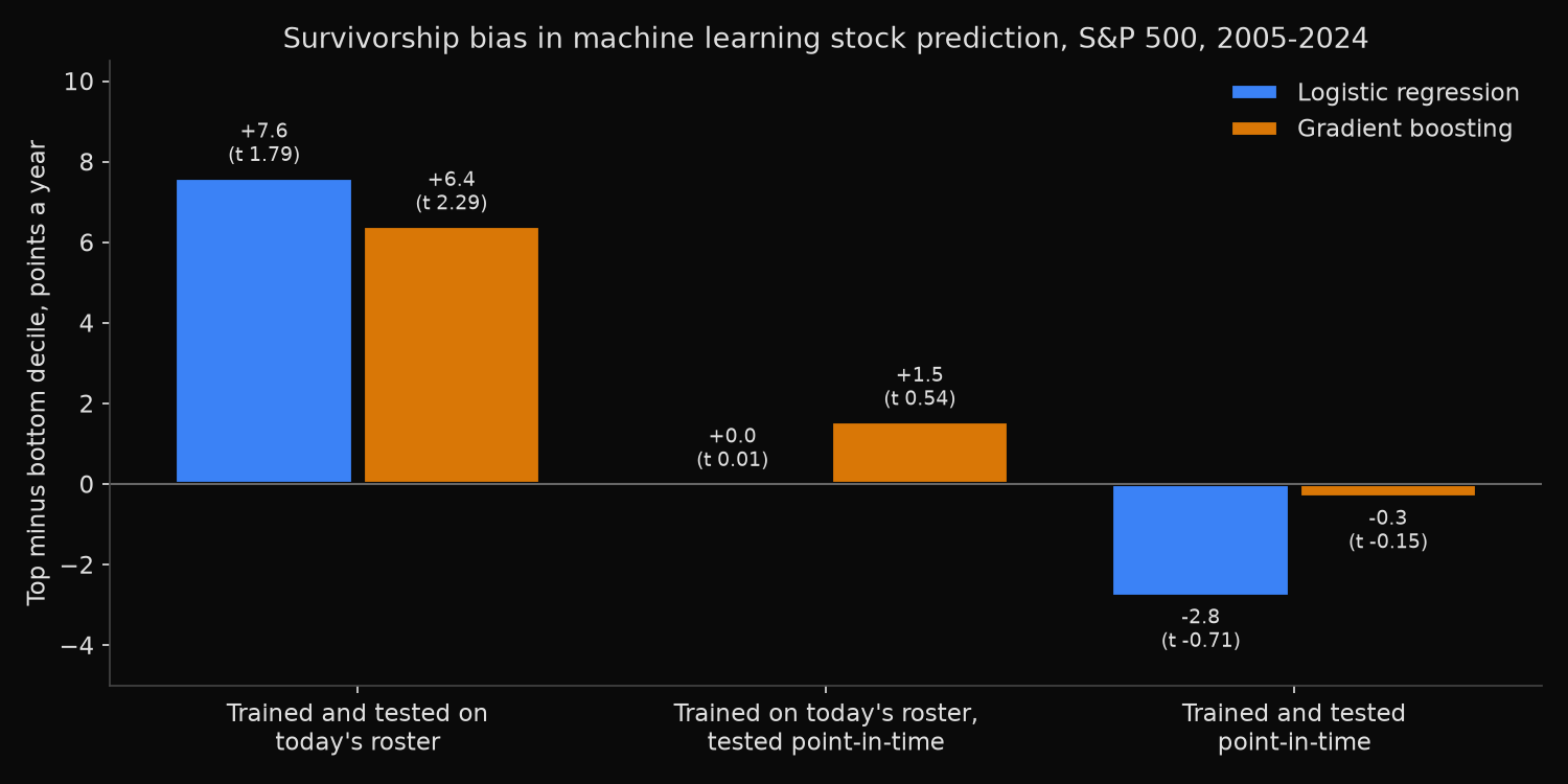
A stock-return model trained on today’s S&P 500 list has its top decile beating its bottom decile by 7.6 points a year from 2005 to 2024 (t 1.79, not significant at 5%), but only when tested on that same list. On the rosters the index actually had, the same logistic regression shows 0.0 points (t-statistic 0.01), and a gradient-boosted version falls from 6.4 points to 1.5 (t 0.54). The survivor list taught both models that volatile, beaten-down stocks win, because the members that later left the index are missing from it.
How does survivorship bias get into a model’s training data?
A return model learns from a panel of company-months (its row structure is the subject of how to build a stock dataset for machine learning). A common shortcut fills that panel from today’s index list, applied to every past month. That list holds survivors and later joiners. Suppose two members each fell 60%: the one that later collapsed has no rows, while the one that recovered keeps all of them. The guide to survivorship bias in backtesting explains the general mechanism.
The hypothesis: a model trained on survivors learns to favour volatile, beaten-down stocks, a preference that earns nothing on the stocks investors could actually buy.
Training two models on two versions of the S&P 500
- Draw the S&P 500 roster at each month end, December 1999 to November 2024, with
xfl.index("sp500", as_of=...)(index membership reference); each sets the next month’s universe. Today’s roster, the same call without a date, had 503 members on 14 November 2026. - Pull monthly total returns for 1,100 securities by
entity_id. A stock that stops trading takes its recorded delisting return in its exit month. - Rank four price-only features within each month’s universe: last month’s return, 12-month momentum skipping the latest month, volatility of the last 12 monthly returns, and distance below the 12-month high.
- Label a row 1 when next month’s return beats that universe’s median, which leaves a pure ranking task.
- Every January from 2005, refit a logistic regression and scikit-learn’s gradient boosting on all labels realised by the prior December. Model A trains on point-in-time rows, model B on today’s-roster rows.
- Sort each month’s universe into deciles by predicted probability, equal-weighted, held one month. Report the top-minus-bottom spread (mean monthly gap times 12), its t-statistic and AUC (the chance a random above-median stock outscores a below-median one; 0.5 is a coin toss).
Code
import numpy as np
import pandas as pd
import xfinlink as xfl
from sklearn.ensemble import HistGradientBoostingClassifier
from sklearn.linear_model import LogisticRegression
from sklearn.metrics import roc_auc_score

xfl.set_api_key("YOUR_API_KEY")  # free at https://xfinlink.com/signup

# Roster on the last business day of each month sets the next month's universe
dates = pd.date_range("1999-12-01", "2024-11-30", freq="BME")
pit = {d.to_period("M") + 1: set(xfl.index("sp500", as_of=d.strftime("%Y-%m-%d"))
                                 .entity_id.dropna().astype(int)) for d in dates}
today = set(xfl.index("sp500").entity_id.dropna().astype(int))
ids = sorted(set().union(*pit.values()) | today)
parts = [xfl.prices(entity_id=ids[i:i + 25], start="1998-12-01", end="2024-12-31",
                    interval="1mo", fields=["return_daily"], max_rows=100_000)
         for i in range(0, len(ids), 25)]
px = pd.concat(parts)
px["m"] = px["date"].dt.to_period("M")
R = px.drop_duplicates(["entity_id", "m"]).pivot(index="m", columns="entity_id", values="return_daily")
R = R.reindex(pd.period_range("1998-12", "2024-12", freq="M"))

# Exits: recorded delisting return in the exit month (one request per exit year, one page each)
last = R.apply(pd.Series.last_valid_index)
ended = last[(last >= pd.Period("1999-12", "M")) & (last < pd.Period("2024-12", "M"))]
delist = {}
for y, g in ended.groupby(ended.map(lambda p: p.year)):
    g = g.index.tolist()
    for i in range(0, len(g), 150):
        d = xfl.prices(entity_id=g[i:i + 150], start=f"{y}-01-01", end="2024-12-31",
                       interval="1mo", fields=["return_daily"])
        delist.update({int(k): v for k, v in (d.attrs["meta"].get("delisting") or {}).items()})
for e, v in delist.items():
    dr = v.get("delisting_return")
    if e in R and dr is not None and not np.isnan(dr):
        m = last[e] if pd.Period(v["event_date"], "M") <= last[e] else last[e] + 1
        if m <= R.index[-1]:
            R.loc[m, e] = (1 + np.nan_to_num(R.loc[m, e])) * (1 + dr) - 1

# Four price-only features known at month end t; the label month is t + 1
lvl = (1 + R.fillna(0)).cumprod()
FEATS = {"ret_1m": R,
         "mom_12_1": np.expm1(np.log1p(R).rolling(11).sum().shift(1)),
         "vol_12m": R.rolling(12).std(),
         "off_high": lvl / lvl.rolling(12).max() - 1}
full = R.rolling(12).count() == 12
X = pd.concat({k: f.where(full).stack() for k, f in FEATS.items()}, axis=1).dropna()
X["y_ret"] = R.shift(-1).stack().reindex(X.index)
X.index.names = ["t", "e"]
X = X.loc["1999-12":"2024-11"].reset_index()
X["hold"] = X["t"] + 1
X["pit"] = [e in pit[h] for e, h in zip(X["e"], X["hold"])]
X["today"] = X["e"].isin(today)
F = list(FEATS)

def universe(col):  # ranks and "beat the median" label, computed inside one universe
    d = X[X[col] & X["y_ret"].notna()].copy()
    g = d.groupby("t")
    d[F] = g[F].rank(pct=True) - 0.5
    d["y"] = (d["y_ret"] > g["y_ret"].transform("median")).astype(int)
    return d

U = {"pit": universe("pit"), "today": universe("today")}
MODELS = {"Logistic regression": lambda: LogisticRegression(C=1.0, max_iter=1000),
          "Gradient boosting": lambda: HistGradientBoostingClassifier(
              max_iter=200, learning_rate=0.05, max_leaf_nodes=15, min_samples_leaf=200,
              early_stopping=False, random_state=0)}

# Walk-forward: refit each January on labels realised by the prior December
pred = []
for y in range(2005, 2025):
    for train in ("pit", "today"):
        tr = U[train][U[train]["hold"].dt.year < y]
        for mdl, make in MODELS.items():
            clf = make().fit(tr[F], tr["y"])
            for test in ("pit", "today"):
                te = U[test][U[test]["hold"].dt.year == y]
                pred.append(te[["t", "e", "y", "y_ret", "today"]].assign(
                    p=clf.predict_proba(te[F])[:, 1], model=mdl, train=train, test=test))
P = pd.concat(pred, ignore_index=True)
P["dec"] = P.groupby(["model", "train", "test", "t"])["p"].transform(
    lambda s: np.ceil(s.rank(pct=True) * 10))

def score(d):
    s = (d[d.dec == 10].groupby("t")["y_ret"].mean() - d[d.dec == 1].groupby("t")["y_ret"].mean())
    return pd.Series({"spread": s.mean() * 12, "t": s.mean() / s.std() * len(s) ** 0.5,
                      "auc": roc_auc_score(d["y"], d["p"])})

print(P.groupby(["model", "train", "test"]).apply(score).round(3))
Full script with formatting and visualisation: machine-learning-stock-prediction-survivorship-bias-python.py
Output
Rosters: 300 month ends, Dec 1999 to Nov 2024; today's roster: 503 names as of 2026-11-14
Securities: 1100; exit months given a recorded delisting return: 430
Rows with features and a label, 2000-2024: point-in-time 149,563, today's roster 125,653
Last month held, point-in-time: ENE 2001-11 -98.1%, WCOM 2002-05 -33.0%, LEH 2008-09 -99.7%, WM 2008-09 -96.0%, FRC 2023-04 -97.6%

Walk-forward test 2005-2024 (240 months), retrained each January
model                trained on      tested on        names     top  bottom  spread      t    AUC rank IC
Gradient boosting    point-in-time   point-in-time      499    9.9%   10.2%   -0.34  -0.15  0.502 +0.0061
Gradient boosting    point-in-time   today's roster     436   14.6%   20.6%   -6.00  -2.63  0.499 -0.0041
Gradient boosting    today's roster  point-in-time      499   10.9%    9.4%   +1.55   0.54  0.503 +0.0051
Gradient boosting    today's roster  today's roster     436   19.5%   13.1%   +6.40   2.29  0.505 +0.0117
Logistic regression  point-in-time   point-in-time      499    9.5%   12.3%   -2.79  -0.71  0.496 -0.0005
Logistic regression  point-in-time   today's roster     436   10.4%   21.9%  -11.57  -3.25  0.491 -0.0172
Logistic regression  today's roster  point-in-time      499   11.1%   11.1%   +0.03   0.01  0.496 -0.0014
Logistic regression  today's roster  today's roster     436   21.1%   13.5%   +7.60   1.79  0.503 +0.0135

Logistic regression coefficients (rank features, mean of 20 yearly fits)
                    ret_1m  mom_12_1   vol_12m  off_high
point-in-time       -0.099    +0.044    -0.100    -0.033
today's roster      -0.162    +0.059    +0.054    -0.105

Training data 2000-2024, next month: share beating the median / mean return a year
  most volatile tenth
    today's roster                  51.7%   32.7%
    point-in-time                   48.4%   11.5%
      still in the index today      51.5%   23.2%
      since removed (58%)           46.2%    3.0%
  tenth furthest below its 12-month high
    today's roster                  51.1%   27.3%
    point-in-time                   48.6%   11.0%
      still in the index today      52.3%   25.2%
      since removed (60%)           46.2%    1.3%

Top decile on the point-in-time universe, 2005-2024: share since removed / volatility rank
  Gradient boosting    trained on point-in-time     31.3%  -0.072
  Gradient boosting    trained on today's roster    39.6%  +0.122
  Logistic regression  trained on point-in-time     24.8%  -0.270
  Logistic regression  trained on today's roster    47.4%  +0.281
What the survivor list taught the model
On the point-in-time universe, model B’s logistic top and bottom deciles both earn 11.1% a year, and the boosted gap of 1.55 points has a t-statistic of 0.54. Model A finds no edge either (−2.79 and −0.34). Every AUC lies between 0.491 and 0.505, within 0.01 of a coin toss; the spreads come from the extremes of each ranking.
Model B’s logistic fit puts +0.054 on volatility where A’s puts −0.100, and −0.105 on distance below the high against −0.033, a pull toward the stocks that have fallen furthest.
The training rows explain why. The most volatile tenth beat the median in 51.7% of survivor-panel rows, returning 32.7% a year over the following month, against 48.4% and 11.5% point-in-time. More than half of the difference is the 58% of that tenth since removed from the index, which returned 3.0% a year against 23.2% for members still there. Stocks furthest below their high split the same way (1.3% for the 60% since removed, 25.2% for the rest). The rest comes from later joiners, whose rows from before they entered the index a survivor panel also keeps.
In testing, that preference picks companies the survivor panel never contained: 47.4% of B’s logistic top decile on the point-in-time universe are companies since removed, against 24.8% for A. Lehman Brothers (−99.7% in September 2008) and First Republic (−97.6% in April 2023) are in the point-in-time rows and absent from the survivor panel.
Checking a return model for survivor-trained habits
Build the training panel from the roster in force on each date, keeping each member, exit return included, until the month it left. The historical S&P 500 constituents lookup shows membership on any past date; as_of returns the same rosters in code. A panel built from today’s list fails silently: the fit and the walk-forward split both look clean.
Score every model on the point-in-time universe and read what it leans on: among large caps, a taste for high volatility or deep drawdowns is what this survivor panel taught. An analysis of stocks removed from the S&P 500 covers how removed members traded before they left.
On the rosters investors faced, these four features gave no reliable edge from 2005 to 2024. The 7.6 points came from the list.
Built with xfinlink — free financial data API for Python.