Look-Ahead Bias in Split-Adjusted Prices, Tested in Python

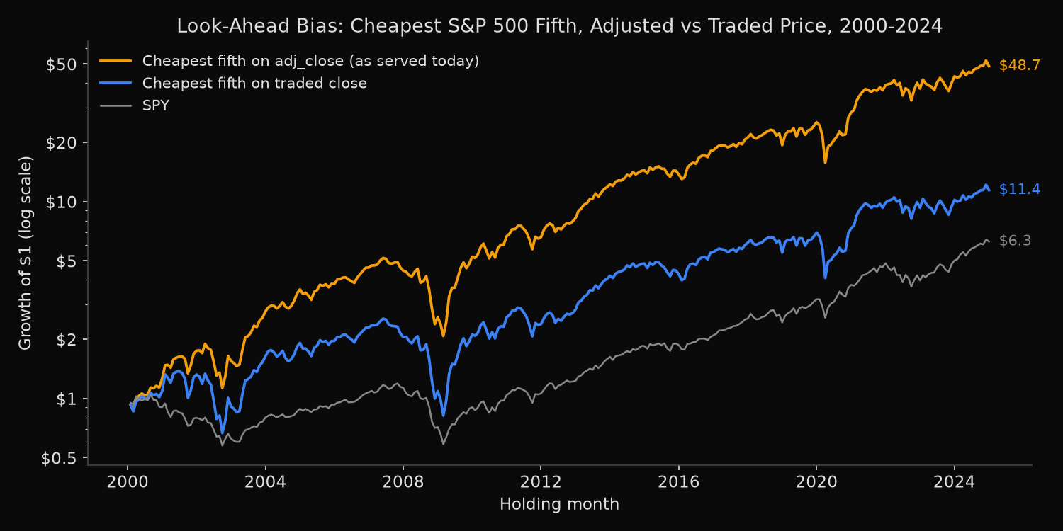
Sorting S&P 500 members on split-adjusted prices leaks the future into a backtest: the cheapest fifth of each month’s roster, picked on adj_close as served today, returned 16.82% a year from 2000 to 2024, against 10.24% when the same rule reads the price that actually traded. Both use the same returns; only the picks differ, and the cheap-minus-dear spread grows from 4.59 points a year (t-statistic 1.26) to 14.80 (t 5.11).

How can a price from 1999 know about a split in 2020?

A split-adjusted price restates every earlier close onto today’s share count. Apple closed 1999 at $102.81; four later splits multiply to 112, so that session now reads $0.918 in adj_close. A return between two dates survives the rescaling, since both prices sit on the same share basis, but a price level does not. A rule that ranks or filters on the level reads a number nobody saw at the time, which is look-ahead bias; the guide to look-ahead bias in backtesting covers the other routes into a test.

Companies split after their shares have risen, so the future winners carry the largest factors and the lowest adjusted prices. William Brown and Ray Pfeiffer (Journal of Business Finance & Accounting, 2007) reported a persistent negative relation between split-adjusted share prices and later returns, and traced about half of a price-sorted hedge return to survivorship and substantially all of the rest to split reclassification.

Two prices for every member on every month end

1. On each month-end trading day from December 1999 to November 2024, draw the roster in force with xfl.index("sp500", as_of=...) (the historical S&P 500 constituents for that date): 300 rosters, 1,062 securities.
2. Take each member’s close (as traded) and adj_close (restated for later splits, stock dividends and spin-offs) on that day. A forward adjustment, compounding split_ratio as the price fields reference shows, has nothing to apply after the formation date, so it equals the traded close there.
3. Rank on each price and hold the cheapest and dearest fifths equal-weight the next month, January 2000 to December 2024, on the same monthly total returns. Members leaving on the formation date are not held (103 member-months), delisting returns enter in the exit month (306 member-months), and members with no return that month drop out (9).
4. Apply “skip anything under $10” to each price and hold what passes.
5. Count picks with close / adj_close above 1 (a later split, stock dividend or spin-off) or below 1 (a later reverse split).

Code

import numpy as np
import pandas as pd
import xfinlink as xfl

xfl.set_api_key("YOUR_API_KEY")  # free at https://xfinlink.com/signup

spy = xfl.prices("SPY", start="1999-12-01", end="2024-12-31", fields=["return_daily"])
spy["date"] = pd.to_datetime(spy["date"])
formation = spy.groupby(spy["date"].dt.to_period("M"))["date"].max().loc[:"2024-11"]

# Roster in force at each month end; a member leaving that day is not held
pit = pd.concat([xfl.index("sp500", as_of=d.strftime("%Y-%m-%d")).dropna(subset=["entity_id"])
                 .assign(month=m, asof=d) for m, d in formation.items()])
pit["entity_id"] = pit["entity_id"].astype(int)
pit = pit[pd.to_datetime(pit["removed_date"]) != pit["asof"]]

# Month-end close (as traded), adj_close (as served today), monthly total return
ids = sorted(pit["entity_id"].unique())
parts, exits = [], {}
for i in range(0, len(ids), 16):   # one page per batch keeps every batch's exit returns
    p = xfl.prices(entity_id=ids[i:i + 16], start="1999-12-01", end="2024-12-31",
                   interval="1mo", fields=["close", "adj_close", "return_daily"],
                   max_rows=100_000)
    parts.append(p)
    exits.update(p.attrs.get("meta", {}).get("delisting", {}) or {})
px = pd.concat(parts)
px["month"] = pd.to_datetime(px["date"]).dt.to_period("M")
bars = px.drop_duplicates(["month", "entity_id"]).set_index(["month", "entity_id"])
ret = px.pivot_table(index="month", columns="entity_id", values="return_daily", aggfunc="first")
for eid, ev in exits.items():      # recorded delisting return, added in the exit month
    eid, dl, m = int(eid), ev.get("delisting_return"), pd.Period(ev["event_date"], "M")
    if dl is not None and eid in ret.columns and m in ret.index:
        r0 = ret.at[m, eid]
        ret.at[m, eid] = (1 + (0 if pd.isna(r0) else r0)) * (1 + dl) - 1

key = pd.MultiIndex.from_arrays([pit["month"], pit["entity_id"]])
pit["close"] = bars["close"].reindex(key).to_numpy()
pit["adj_close"] = bars["adj_close"].reindex(key).to_numpy()
pit["r"] = ret.stack().reindex(pd.MultiIndex.from_arrays(
    [pit["month"] + 1, pit["entity_id"]])).to_numpy()   # next month's return; no fill
book = pit.dropna(subset=["close", "adj_close"]).copy()
for col in ("close", "adj_close"):
    book["q_" + col] = book.groupby("month")[col].transform(
        lambda s: pd.qcut(s.rank(method="first"), 5, labels=False) + 1)
held = book.dropna(subset=["r"])

ann = lambda r: ((1 + r).prod() ** (12 / len(r)) - 1) * 100
for col in ("close", "adj_close"):
    g = held.groupby(["month", "q_" + col])["r"].mean().unstack()
    d = g[1] - g[5]
    print(col, f"cheapest {ann(g[1]):.2f}%", f"dearest {ann(g[5]):.2f}%",
          f"spread {d.mean() * 1200:.2f}", f"t {d.mean() / d.std() * np.sqrt(len(d)):.2f}")
for col in ("close", "adj_close"):  # "skip anything under $10", applied to each price
    print(col, "$10+ filter", f"{ann(held[held[col] >= 10].groupby('month')['r'].mean()):.2f}%")

Full script with formatting and visualisation: lookahead-bias-split-adjusted-prices-python.py

Output

300 month ends, 1062 securities, holding months 2000-01 to 2024-12
Member-months sorted: 150,418; not held because the member left on the formation date: 103; no month-end price: 0; no return in the holding month: 9; held member-months with a recorded delisting return: 306

Equal-weight quintiles sorted on month-end price, held the next month
                 cheapest fifth % a year  dearest fifth % a year  cheap minus dear, points a year  t-stat
sort on                                                                                                  
as traded                          10.24                    7.79                             4.59    1.26
as served today                    16.82                    2.45                            14.80    5.11
SPY over the same 300 months: 7.62% a year
Cheapest fifth, served minus traded: +5.23 points a year, t-stat 6.49, served version ahead in 66% of 300 months
Cheapest-fifth picks that differ between the two sorts: 28 of 100 a month

                           % restated up later  median factor if so  % reverse split later
cheapest fifth, as traded                10.74                 1.33                   9.57
cheapest fifth, as served                37.35                 3.28                   1.24
dearest fifth, as traded                 41.54                 2.00                   0.67
dearest fifth, as served                 12.61                 1.18                   8.27
by five-year period, cheapest fifth served minus traded, points a year: 2000-2004 +11.11, 2005-2009 +4.87, 2010-2014 +3.45, 2015-2019 +3.88, 2020-2024 +2.86

Under-$10 filter, member-months: served price under $10 but traded at $10 or more: 4,026 (131 securities); the reverse: 1,222 (37 securities); total held 150,409
  next-month return, mean: wrongly skipped 2.28%, wrongly kept 0.21%, passing on both prices 0.81%
  equal-weight members priced $10 or more: as traded 9.32% a year, as served today 8.68% a year; difference -0.57 points a year, t-stat -6.33
  all members, no filter: 9.80% a year

As traded vs as served today
ticker       date    close  adj_close  factor  fifth traded  fifth served
  AAPL 1999-12-31 102.8125     0.9180   112.0             5             1
  NVDA 2001-11-30  54.6400     0.4553   120.0             5             1
Months AAPL sat in the served cheapest fifth while in the traded top two fifths: 148

A look-ahead bias example: later splits sort the winners into the cheap fifth

On traded prices the spread, 4.59 points a year at t 1.26, is not statistically significant; on adjusted prices it is 14.80 (t 5.11). The served cheapest fifth compounds 6.58 points a year ahead of the traded one, and its monthly lead (5.23 points a year, t 6.49) averages positive in every five-year period, from 11.11 points in 2000-2004 to 2.86 in 2020-2024.

The picks that differ, about 28 of 100 a month, carry the later splits: 37.35% of the served cheapest fifth were later restated upward, at a median factor of 3.28, against 10.74% and 1.33 as traded. Apple sat in the served cheapest fifth for 148 months while in the top two fifths as traded; NVIDIA closed at $54.64 on 30 November 2001 and now reads $0.455. At the dear end, 8.27% of the served fifth later reverse-split, against 0.67% as traded, and that bucket sinks to 2.45% a year.

The $10 filter errs the other way. In 4,026 member-months across 131 securities, a stock traded at $10 or more but reads below $10 today; those names averaged 2.28% the next month, against 0.81% for members above $10 on both prices. On net, the served filter trails the traded one by 0.57 points a year (t -6.33). The sign depends on the rule: buying low adjusted prices flatters a test, excluding them penalises it.

Which price a rule on price levels should read

A rule that compares a price level with a threshold or with other stocks should read the close that traded on the formation date. Price ranks, $5 and $10 floors and price as a ratio’s denominator are exposed; returns, volatility and moving-average crossovers can stay on adj_close, because the factor cancels. Running a test on both columns is a cheap check: if the answer moves, the rule reads a level.

Each new split restates adj_close again, so a level-based backtest on it drifts over time. The universe needs the same dating as the price, and the history of S&P 500 additions and deletions sets out how the index’s membership changes are logged by date.

Built with xfinlink — free financial data API for Python.