
To backtest a stock strategy, write the rule down first, replay it through history using only the companies, prices and costs available on each date, and compare the result with something you could have bought instead. Those steps decide the answer: one 50-stock momentum rule on S&P 500 members earns 8.51% a year from 2000 to 2024 when every step is done properly, and 21.10% a year when the only change is using today’s index list. The seven steps below build the correct version in Python, and the table after them prices each shortcut.
What does it mean to backtest a stock strategy?
A backtest applies a fixed trading rule to past data and records what the rule would have earned. Its value is narrow but real: it can reject an idea cheaply, before any money depends on it. It cannot prove that an idea will work, since the future may not resemble the sample, and it reports nonsense without any warning when the inputs carry information nobody had at the time.
The example here is a teaching vehicle rather than a recommendation. Momentum, the tendency of recent winners to keep winning, makes a good subject because the rule fits in one sentence and every common error can damage it.
Step 1: What exactly does the rule say?
A rule is testable when two people coding it separately would buy the same stocks. “Buy strong stocks” fails that standard, and this version passes:
- At each month end, take the S&P 500 members on that date.
- Rank them by price change over the six months that ended one month earlier.
- Buy the top 50 at equal weight and hold them for one month.
- Charge 10 basis points (0.10%) on every dollar bought or sold.
Fix these terms before looking at any result. Each change made after seeing an equity curve fits the rule a little more closely to the past, an error known as overfitting, and step 7 tests for it.
Step 2: Which stocks were available on each date?
Use the members of the universe on each past date, including the ones that later failed. Today’s index list has already dropped them: 188 of the 500 members from December 1999 remain on it. Testing on that list is survivorship bias, and it fills the early years with companies that only joined because they later grew.
from concurrent.futures import ThreadPoolExecutor
import pandas as pd
import xfinlink as xfl

xfl.set_api_key("YOUR_API_KEY")  # free at https://xfinlink.com/signup

days = pd.to_datetime(xfl.prices("SPY", start="1999-12-01", end="2024-12-31", fields=["close"])["date"])
month_ends = days.groupby(days.dt.to_period("M")).max()

def roster(d):
    return d.to_period("M"), set(xfl.index("sp500", as_of=d.strftime("%Y-%m-%d")).entity_id.dropna().astype(int))

with ThreadPoolExecutor(8) as pool:
    dated = dict(pool.map(roster, month_ends))
Each as_of call returns one date’s members, with those later removed or delisted still on the list; the index membership reference gives the parameters. To read a roster without code, the historical S&P 500 constituents lookup shows the members on any date, and the dated history of additions and deletions sets out the changes between rosters.
Step 3: Which prices and returns should the backtest use?
Three column choices matter here. Rank on adj_close, which a split cannot distort. Earn return_daily, which on monthly bars is the total return for the month, dividends included. Key everything on entity_id rather than the ticker, because tickers get reused: MIR meant Mirage Resorts until May 2000 and Mirant from January 2001 to July 2003, and both companies appear on these rosters.
The last piece is what a holder received when a stock left the market. Each response from the prices endpoint carries the recorded exits for its securities in meta.delisting.
ids = sorted(set().union(*dated.values()))

def fetch(i):
    df = xfl.prices(entity_id=ids[i:i + 12], start="1999-01-01", end="2024-12-31", interval="1mo",
                    fields=["adj_close", "return_daily"], max_rows=100_000)
    return df, df.attrs["meta"].get("delisting") or {}

with ThreadPoolExecutor(8) as pool:
    batches = list(pool.map(fetch, range(0, len(ids), 12)))

px = pd.concat(b[0] for b in batches).astype({"entity_id": int})
px["month"] = pd.to_datetime(px["date"]).dt.to_period("M")
close = px.pivot(index="month", columns="entity_id", values="adj_close")
returns = px.pivot(index="month", columns="entity_id", values="return_daily")

for _, exits in batches:  # add each recorded exit return to the final month
    for i, ev in exits.items():
        month = pd.Period(ev["event_date"][:7], "M")
        if ev["delisting_return"] is not None and month in returns.index:
            last = returns.loc[month, int(i)]
            returns.loc[month, int(i)] = (1 + (0 if pd.isna(last) else last)) * (1 + ev["delisting_return"]) - 1
Step 4: When could the trade really have happened?
A signal may only use data that existed before the trade. Nobody can rank stocks on a closing price and also buy at that same close, and monthly bars cannot express a one-day delay, so the rule leaves a full month between the last close it ranks on and the trade. The look-ahead error usually comes from something smaller than bad intent: one shifted index in a table. The guide to look-ahead bias covers the other common source, financial figures used before their filing date.
signal = close / close.shift(6) - 1
months = sorted(dated)[:-1]

def backtest(cost_bp=10):
    out, weights = {}, pd.Series(dtype=float)
    for t in months:
        ranks = signal.loc[t - 1].reindex(sorted(dated[t])).dropna()      # ends one month before the trade
        ranks = ranks[close.loc[t].reindex(ranks.index).notna()]          # has a bar in the trade month
        picks = ranks.nlargest(50).index
        target = pd.Series(1 / 50, index=picks)
        both = target.index.union(weights.index)
        traded = (target.reindex(both, fill_value=0) - weights.reindex(both, fill_value=0)).abs().sum()
        r = returns.loc[t + 1].reindex(picks).fillna(0)                   # a finished series sits in cash
        out[t + 1] = (target * r).sum() - traded * cost_bp / 10_000
        weights = target * (1 + r) / (target * (1 + r)).sum()
    return pd.Series(out)

strategy = backtest()
Step 5: What would the trades have cost?
Every trade pays part of the bid-ask spread and some slippage, the gap between the price assumed and the price obtained, and often a commission. The cost depends on how much the rule trades. This one replaces a large part of its book each month: buys and sells together average 83% of the portfolio, so a 10-basis-point charge removes 1.07 points a year, the difference between 9.58% and 8.51%. Ten basis points is an assumption for large US stocks, not a measurement. A rule that trades smaller companies should test a higher figure.
Step 6: Did the strategy beat something you could have bought?
An absolute return says little until it stands next to an alternative that was available at the time. Two comparisons apply here: SPY with dividends, which anyone could have held, and an equal-weight portfolio of all ranked members, charged the same 10 basis points, which uses the same universe and shows what the selection added. The guide to picking a backtest benchmark explains how to match one to a strategy.
Read at least three numbers. Annual return gives the compound growth rate, return/risk divides average return by volatility (a Sharpe ratio with no risk-free rate subtracted), and maximum drawdown records the worst fall from a previous high. A strategy can look good on one and fail the others.
def stats(r):
    wealth = (1 + r).cumprod()
    return {"% a year": (wealth.iloc[-1] ** (12 / len(r)) - 1) * 100,
            "volatility %": r.std() * 12 ** 0.5 * 100,
            "return/risk": r.mean() / r.std() * 12 ** 0.5,
            "max drawdown %": (wealth / wealth.cummax() - 1).min() * 100,
            "$1 becomes": wealth.iloc[-1]}

bars = xfl.prices("SPY", start="2000-01-01", end="2024-12-31", interval="1mo", fields=["return_daily"])
spy = bars.set_index(pd.to_datetime(bars["date"]).dt.to_period("M"))["return_daily"].reindex(strategy.index)
print(pd.DataFrame({"Correct version": stats(strategy), "SPY, total return": stats(spy)}).T.round(2))
Full script with the variants and the chart: how-to-backtest-a-stock-strategy.py
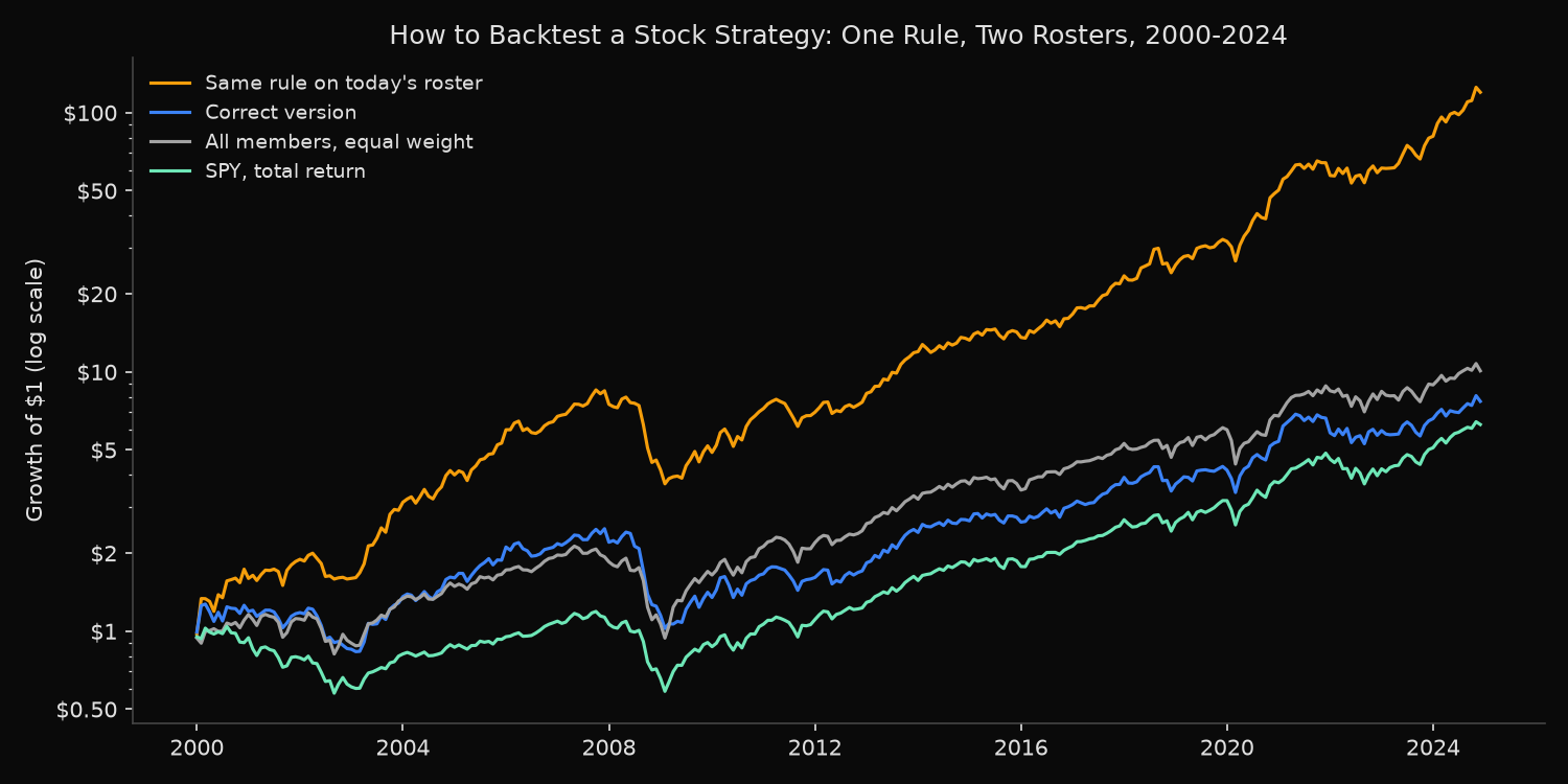
Output (full script):
                                     % a year  volatility %  return/risk  max drawdown %   $1 becomes
Correct version                          8.51         19.22         0.52          -58.78         7.70
SPY, total return                        7.62         15.26         0.56          -50.80         6.27
All members, equal weight                9.69         17.68         0.61          -55.80        10.10
The correct version beats SPY on return by 0.89 points a year, and it pays for that with a deeper drawdown (-58.78% against -50.80%) and a slightly lower return/risk (0.52 against 0.56). It trails the plain equal-weight portfolio of its own universe by 1.18 points. Over the full period, ranking the members added nothing measurable, and the gap is well within its noise.
How much does each shortcut change the result?
Each row below makes one change to the correct version.
| Shortcut | % a year | Change (points) |
|---|---|---|
| None (correct version) | 8.51 | |
| Today’s roster instead of dated rosters | 21.10 | +12.59 |
| Ranks on the holding month itself | 101.04 | +92.53 |
| Fills at the close it ranked on | 8.27 | -0.24 |
| Price return, no dividends or exit returns | 7.26 | -1.25 |
| No trading costs | 9.58 | +1.07 |
| No exit returns | 8.52 | +0.01 |
Two of the errors cost more to miss than the rest, for opposite reasons. Ranking on the holding month produces 101% a year, which no one would believe, so the code gets checked. Today’s roster produces 21.10% with a return/risk of 1.01, a figure that looks like a very good strategy rather than a bug, and it would have turned $1 into about $120 instead of $7.70.
Shortcuts do not all flatter. Dropping dividends lowers the result, as does filling at the ranking close here, so the direction of an error is not always obvious in advance. Exit returns barely move this rule because few of its positions ended that way: 97 of 15,000, and 93 of those were mergers, where the median final move across all recorded mergers is 0.11%. The rule held only two of the 54 exchange removals, whose median final move is -45.41%, and a portfolio holding more of those names should book the loss.
Step 7: How do you know the result is not luck?
Three checks follow, and this rule passes none of them.
Split the sample. Choose the rule on one period and judge it on another. The 2000-2012 half beats SPY, 4.20% a year against 1.60%, and anyone stopping there would have felt encouraged. In 2013-2024 it trails, 13.37% against 14.54%. Walk-forward testing extends the same idea by repeatedly fitting on a window and testing on the period after it.
Move the parameters. A real effect should survive small changes.
Parameter grid, % a year after costs (rows: holdings; columns: lookback months)
        3     6     9
25   6.73  7.06  7.75
50   6.98  8.51  8.10
100  7.09  8.64  8.45
No combination reaches the 9.69% of the equal-weight portfolio. Five of the nine cells beat SPY and four do not, so the lead over SPY depends on the settings. This grid shows no isolated spike, which would point to fitting; the failure is that the edge itself does not hold up.
Measure the gap against its noise. The rule’s average lead over SPY is 1.49 points a year, with a t-statistic of 0.59, and it finished ahead in 156 of 300 months. A t-statistic below about 2 means the gap cannot be told apart from chance. (The 1.49 is an arithmetic average, which is why it exceeds the 0.89 compound difference.) Count independent periods rather than trades here: 15,000 positions sound like a large sample, but they came from 300 monthly bets on overlapping stocks.
A rule that passes these checks moves on to paper trading, where it runs on live prices with no money at risk, then to a small live position. This one stops here, which is what a backtest is for.
Do you need a backtesting library?
For a monthly portfolio like this one, the pandas loop in step 4 is enough. Libraries suit different work. Backtesting.py’s own guide says it “doesn’t really support stock picking” or multi-asset rebalancing and “works with an individual tradeable asset at a time”, and tells users “You bring your own data” (as of November 2026). That makes it a fit for a rule on one instrument. Backtrader’s data-feed documentation lists CSV-based parsers, including Yahoo files and generic CSV, each reading a file or ticker the user supplies (also as of November 2026).
Either way the tool simulates the trades on whatever it receives. The list of companies that belonged in the test on each date still has to come from the data.
Where do you get the data for a full run?
The code above makes about 1,400 requests and returns about 232,000 monthly rows, which fits inside a Pro key’s daily limits. A free key reads the last 12 months of prices, one security a request, and serves rosters for past dates, which is enough to test the joins on a handful of names before paying for anything; the 25-year test needs a paid plan, listed on the pricing page.
FAQ
Is backtesting accurate?
It is as accurate as its inputs, and it measures the past only. The same rule here reads 8.51% or 21.10% a year depending on one input, the roster.
How long should a backtest be?
Long enough to include at least one bear market the rule was not designed around. This window contains 2000-2002, 2008 and March 2020.
Can you backtest a stock strategy without coding?
Yes, spreadsheets and no-code platforms can replay a rule. Ask the same question of each one: does its universe include companies that were later removed from the market?
Does a good backtest mean the strategy will work?
No. It means the idea survived a test it could have failed. Costs, capacity and changing markets still decide what happens with real money.
*Built with xfinlink — free financial data API for Python. pip install -U xfinlink*